Project 1 - Data Cleaning and Transformation using Pivot table and Charts for the Report on requirement of Team Hiring

a. Do proper formatting of the data with using borders, font size and appropriate alignment of the content.

Used Formatting styles

Borders : All borders
Font size = 11
header font size = 11
Headers = Bold
align = center align

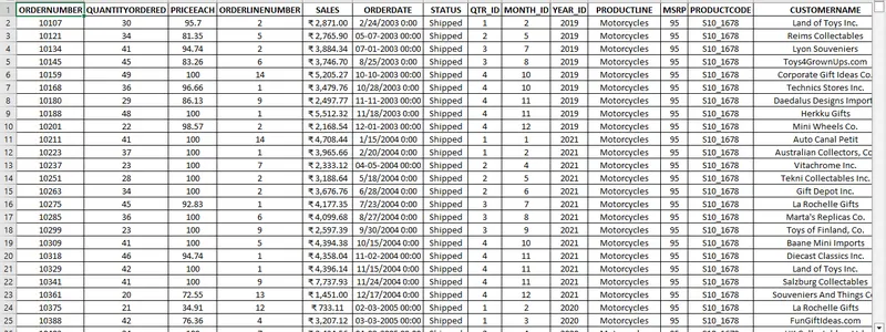
sheetname : a

b. Make summary of Products Sales by providing

1. Total Sum of Sales
2. Average of Sales
3. Standard Deviation of Sales
4. Variance of Sales
5. Maximum Sales
6. Minimum Sales

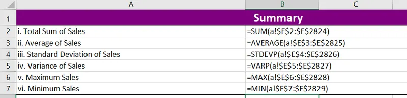
I used Below formulae to get the summary (sheetname = b)

Summary
i. Total Sum of Sales	=SUM(a!$E$2:$E$2824)
ii. Average of Sales	=AVERAGE(a!$E$3:$E$2825)
iii. Standard Deviation of Sales	=STDEVP(a!$E$4:$E$2826)
iv. Variance of Sales	=VARP(a!$E$5:$E$2827)
v. Maximum Sales	=MAX(a!$E$6:$E$2828)
vi. Minimum Sales	=MIN(a!$E$7:$E$2829)

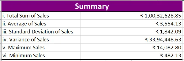
Result:

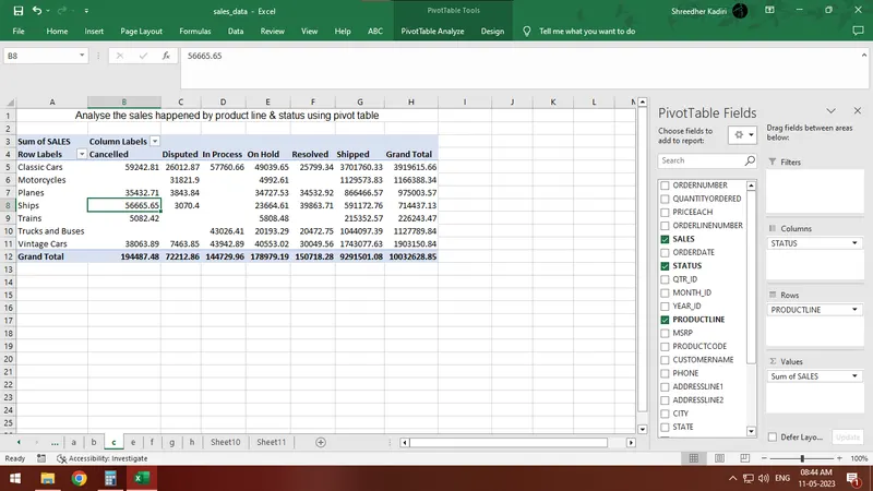
c. Analyse the sales happened by product line & status using pivot table

sheet name : c

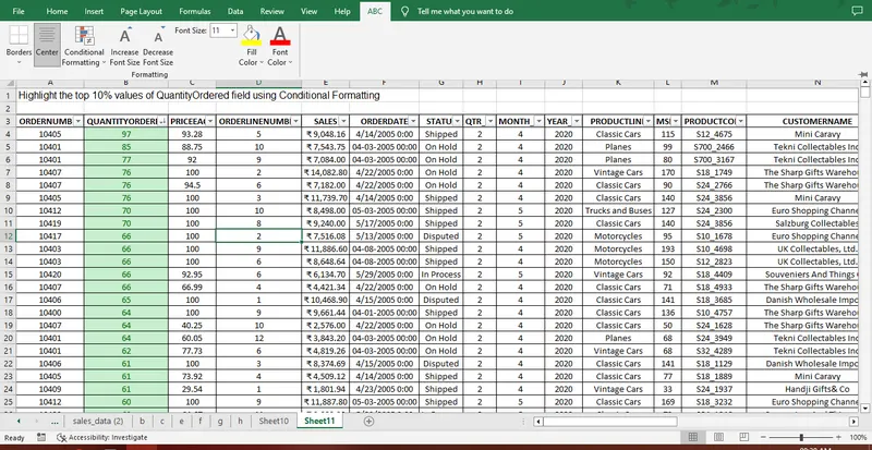
d. Make Customized Tab by naming ABC and keep few data formatting commands in the newly created Tab.

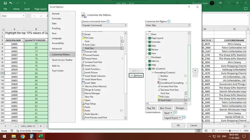
using the Customize ribbon in thee options I added some formatting functionalities to ABC ribbon tab

e. Analyse the Quantities ordered by each Country in Year 2019,2020 and 2021 for different Quarters using Pivot Table.

I have used here two kinds of pivot charts one with the filters and another without filters option

I prefer to use the first one from the left.

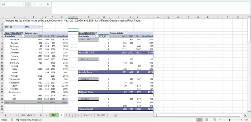
I used filters for filtering quarter ordered, year of order dates in the columns and Countries in the rows

and values field is used to get the sum of orderedquantities using Pivot table

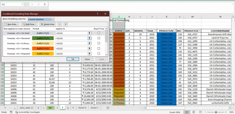
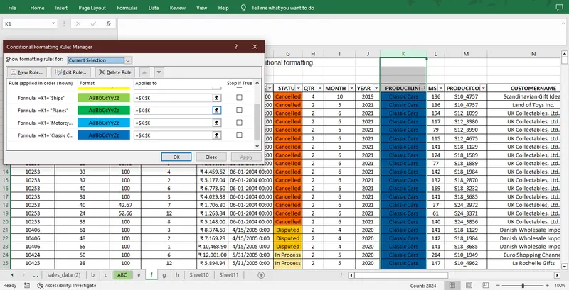
f. Present the data in different colours for values in field Status and ProductLine using conditional formatting.

sheet_name : f

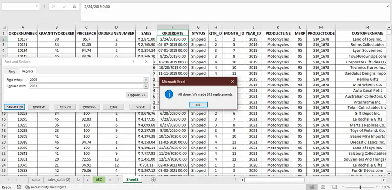
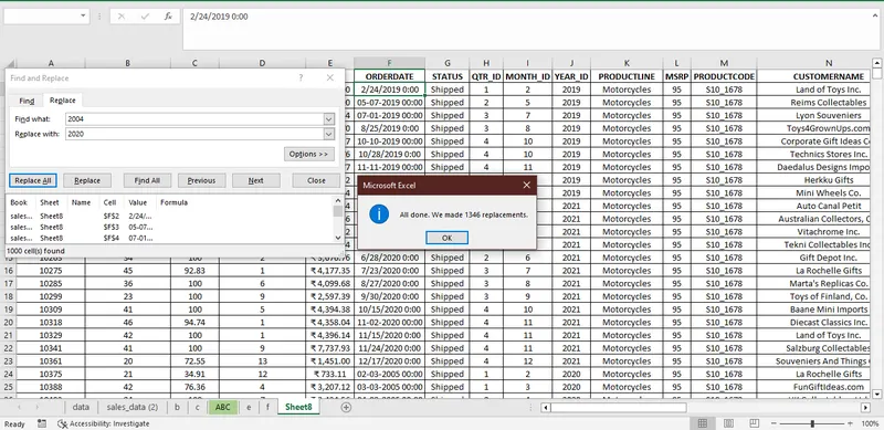
g. change values of 2003 to 2019, 2004 to 2020 and 2005 to 2021 by using proper date formatting options.

sheet_name : g (renamed)

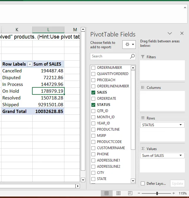
h. Calculate the total sales of all “Shipped”, “Cancelled”, “Disputed”, “In Process”, “On Hold”, “Resolved” products. (Hint:Use pivot table or sumif function)

sheet_name : h

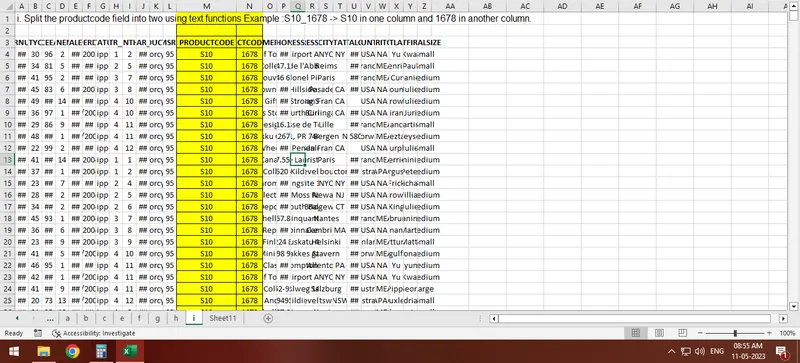
i. Split the productcode field into two using text functions Example :S10_1678 -> S10 in one column and 1678 in another column.

sheet_name : i

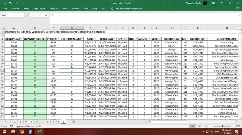
j. Highlight the top 10% values of QuantityOrdered field using Conditional Formatting

The result shows the top 10% , 2824 records ie,. 304 records are highlighted and filtered in the descending order in the sheet

sheet_name = j