Challenge

Project 1

SSai Sumanth Siddam Reddy11 Oct 2022

|| Predicting the Heart Disease in Patients ||

Supposing as appointed as the Data Scientist in a pharma company and our company makes medicine for heart disease patients.

As given several clinical parameters about a patient by my senior manager, I predicted whether the patient has heart disease or not. Those clinical paramters include -

1. age - age in years
2. sex - (1 = male; 0 = female)
3. cp - chest pain type

0: Typical angina: chest pain related decrease blood supply to the heart
1: Atypical angina: chest pain not related to heart
2: Non-anginal pain: typically esophageal spasms (non heart related)
3: Asymptomatic: chest pain not showing signs of disease

4. trtbps - resting blood pressure (in mm Hg on admission to the hospital) anything above 130-140 is typically cause for concern
5. chol - serum cholestoral in mg/dl

serum = LDL + HDL + .2 * triglycerides
above 200 is cause for concern

6. fbs - (fasting blood sugar > 120 mg/dl) (1 = true; 0 = false)

'>126' mg/dL signals diabetes

7. restecg - resting electrocardiographic results

0: Nothing to note
1: ST-T Wave abnormality
- 1. can range from mild symptoms to severe problems
- 2. signals non-normal heart beat
2: Possible or definite left ventricular hypertrophy
- 1. Enlarged heart's main pumping chamber

8. thalachh - maximum heart rate achieved

9. exng - exercise induced angina (1 = yes; 0 = no)

10. oldpeak - ST depression induced by exercise relative to rest looks at stress of heart during excercise unhealthy heart will stress more

11. slp - the slope of the peak exercise ST segment

0: Upsloping: better heart rate with excercise (uncommon)
1: Flatsloping: minimal change (typical healthy heart)
2: Downslopins: signs of unhealthy heart

12. caa - number of major vessels (0-3) colored by flourosopy

colored vessel means the doctor can see the blood passing through
the more blood movement the better (no clots)

13. thall - thalium stress result

1,3: normal
6: fixed defect: used to be defect but ok now
7: reversable defect: no proper blood movement when excercising

14. output - have disease or not (1=yes, 0=no) (= the predicted attribute)

When you working on the health of patients then accuracy is deciding factor, Applying different machine learning algorithms and checked the accuracy about predicting whether or not the patient has heart disease.

Prediction on getting attacked by Heart Disease

A heart attack (Cardiovascular diseases) occurs when the flow of blood to the heart muscle suddenly becomes blocked. From WHO statistics every year 17.9 million dying from heart attack. The medical study says that human life style is the main reason behind this heart problem. Apart from this there are many key factors which warns that the person may/maynot getting chance of heart attack.

This dataset contain some medical information of patients which tells whether that person getting a heart attack chance is less or more. Using the information explore the dataset and classify the target variable using different Machine Learning models and findout which algorithm suitable for this dataset.

Importing Libraries

In [186]:

import numpy as np
import pandas as pd
import matplotlib.pyplot as plt
from sklearn.preprocessing import StandardScaler
from sklearn.model_selection import train_test_split
from sklearn.ensemble import RandomForestClassifier
from sklearn.tree import DecisionTreeClassifier
from sklearn.linear_model import LogisticRegression
from sklearn.svm import SVC
from sklearn.neighbors import KNeighborsClassifier
from sklearn.metrics import mean_squared_error,accuracy_score,confusion_matrix
import seaborn as sns

Loading Dataset

In [25]:

data = pd.read_csv(r'C:\Users\Sumanth Reddy\OneDrive\Documents\datasets\heart.csv',na_values='?')

In [26]:

data

Out[26]:

	age	sex	cp	trtbps	chol	fbs	restecg	thalachh	exng	oldpeak	slp	caa	thall	output
0	63	1	3	145	233	1	0	150	0	2.3	0	0	1	1
1	37	1	2	130	250	0	1	187	0	3.5	0	0	2	1
2	41	0	1	130	204	0	0	172	0	1.4	2	0	2	1
3	56	1	1	120	236	0	1	178	0	0.8	2	0	2	1
4	57	0	0	120	354	0	1	163	1	0.6	2	0	2	1
...	...	...	...	...	...	...	...	...	...	...	...	...	...	...
298	57	0	0	140	241	0	1	123	1	0.2	1	0	3	0
299	45	1	3	110	264	0	1	132	0	1.2	1	0	3	0
300	68	1	0	144	193	1	1	141	0	3.4	1	2	3	0
301	57	1	0	130	131	0	1	115	1	1.2	1	1	3	0
302	57	0	1	130	236	0	0	174	0	0.0	1	1	2	0

303 rows × 14 columns

In [27]:

data.head()

Out[27]:

	age	sex	cp	trtbps	chol	fbs	restecg	thalachh	exng	oldpeak	slp	thall	output
0	63	1	3	145	233	1	0	150	0	2.3	0	1	1
1	37	1	2	130	250	0	1	187	0	3.5	0	2	1
2	41	0	1	130	204	0	0	172	0	1.4	2	2	1
3	56	1	1	120	236	0	1	178	0	0.8	2	2	1
4	57	0	0	120	354	0	1	163	1	0.6	2	2	1

In [28]:

data.tail()

Out[28]:

	age	sex	cp	trtbps	chol	fbs	restecg	thalachh	exng	oldpeak	slp	caa	thall
298	57	0	0	140	241	0	1	123	1	0.2	1	0	3
299	45	1	3	110	264	0	1	132	0	1.2	1	0	3
300	68	1	0	144	193	1	1	141	0	3.4	1	2	3
301	57	1	0	130	131	0	1	115	1	1.2	1	1	3
302	57	0	1	130	236	0	0	174	0	0.0	1	1	2

In [29]:

data.info()

<class 'pandas.core.frame.DataFrame'>
RangeIndex: 303 entries, 0 to 302
Data columns (total 14 columns):
 #   Column    Non-Null Count  Dtype  
---  ------    --------------  -----  
 0   age       303 non-null    int64  
 1   sex       303 non-null    int64  
 2   cp        303 non-null    int64  
 3   trtbps    303 non-null    int64  
 4   chol      303 non-null    int64  
 5   fbs       303 non-null    int64  
 6   restecg   303 non-null    int64  
 7   thalachh  303 non-null    int64  
 8   exng      303 non-null    int64  
 9   oldpeak   303 non-null    float64
 10  slp       303 non-null    int64  
 11  caa       303 non-null    int64  
 12  thall     303 non-null    int64  
 13  output    303 non-null    int64  
dtypes: float64(1), int64(13)
memory usage: 33.3 KB

In [30]:

data.describe().T

Out[30]:

	count	mean	std	min	25%	50%	75%	max
age	303.0	54.366337	9.082101	29.0	47.5	55.0	61.0	77.0
sex	303.0	0.683168	0.466011	0.0	0.0	1.0	1.0	1.0
cp	303.0	0.966997	1.032052	0.0	0.0	1.0	2.0	3.0
trtbps	303.0	131.623762	17.538143	94.0	120.0	130.0	140.0	200.0
chol	303.0	246.264026	51.830751	126.0	211.0	240.0	274.5	564.0
fbs	303.0	0.148515	0.356198	0.0	0.0	0.0	0.0	1.0
restecg	303.0	0.528053	0.525860	0.0	0.0	1.0	1.0	2.0
thalachh	303.0	149.646865	22.905161	71.0	133.5	153.0	166.0	202.0
exng	303.0	0.326733	0.469794	0.0	0.0	0.0	1.0	1.0
oldpeak	303.0	1.039604	1.161075	0.0	0.0	0.8	1.6	6.2
slp	303.0	1.399340	0.616226	0.0	1.0	1.0	2.0	2.0
caa	303.0	0.729373	1.022606	0.0	0.0	0.0	1.0	4.0
thall	303.0	2.313531	0.612277	0.0	2.0	2.0	3.0	3.0
output	303.0	0.544554	0.498835	0.0	0.0	1.0	1.0	1.0

In [31]:

data.columns

Out[31]:

Index(['age', 'sex', 'cp', 'trtbps', 'chol', 'fbs', 'restecg', 'thalachh',
       'exng', 'oldpeak', 'slp', 'caa', 'thall', 'output'],
      dtype='object')

In [32]:

data.dtypes

Out[32]:

age           int64
sex           int64
cp            int64
trtbps        int64
chol          int64
fbs           int64
restecg       int64
thalachh      int64
exng          int64
oldpeak     float64
slp           int64
caa           int64
thall         int64
output        int64
dtype: object

In [33]:

data.isnull().sum()

Out[33]:

age         0
sex         0
cp          0
trtbps      0
chol        0
fbs         0
restecg     0
thalachh    0
exng        0
oldpeak     0
slp         0
caa         0
thall       0
output      0
dtype: int64

In [34]:

data.nunique()

Out[34]:

age          41
sex           2
cp            4
trtbps       49
chol        152
fbs           2
restecg       3
thalachh     91
exng          2
oldpeak      40
slp           3
caa           5
thall         4
output        2
dtype: int64

In [35]:

data.value_counts()

Out[35]:

age  sex  cp  trtbps  chol  fbs  restecg  thalachh  exng  oldpeak  slp  caa  thall  output
38   1    2   138     175   0    1        173       0     0.0      2    4    2      1         2
59   1    0   110     239   0    0        142       1     1.2      1    1    3      0         1
          2   126     218   1    1        134       0     2.2      1    1    1      0         1
          1   140     221   0    1        164       1     0.0      2    0    2      1         1
          0   170     326   0    0        140       1     3.4      0    0    3      0         1
                                                                                             ..
51   1    2   94      227   0    1        154       1     0.0      2    1    3      1         1
          0   140     299   0    1        173       1     1.6      2    0    3      0         1
                      298   0    1        122       1     4.2      1    3    3      0         1
                      261   0    0        186       1     0.0      2    0    2      1         1
77   1    0   125     304   0    0        162       1     0.0      2    3    2      0         1
Length: 302, dtype: int64

In [62]:

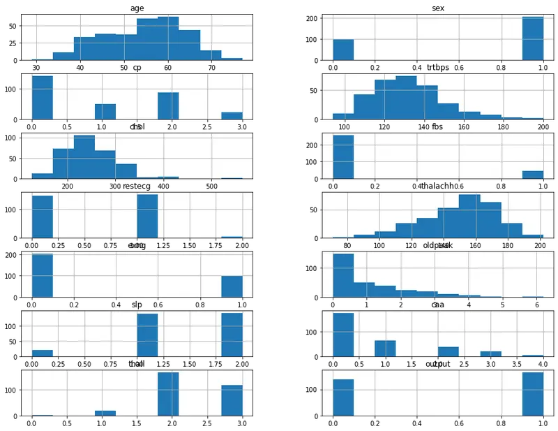
diagram=data.hist(figsize=(15,15),layout=(9,2))

In [63]:

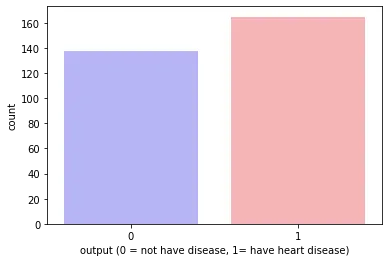
# Checking the number of patients who have disease or not
data['output'].value_counts()

Out[63]:

1    165
0    138
Name: output, dtype: int64

In [67]:

sns.countplot(x='output',data=data,palette='bwr')
plt.xlabel("output (0 = not have disease, 1= have heart disease)")
plt.show()

In [93]:

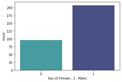
countFemale = len(data[data.sex==0])
countmale = len(data[data.sex==1])

print("Percentage of Female Patients: {:.2f}%".format((countFemale / (len(data.sex))*100)))
print('-'*35)
print("Percentage of Male Patients : {:.2f}%".format((countmale/ (len(data.sex))*100)))

Percentage of Female Patients: 31.68%
-----------------------------------
Percentage of Male Patients : 68.32%

In [91]:

sns.countplot(x='sex',data=data,palette="mako_r")
plt.xlabel('Sex (0:Female , 1 : Male)')
plt.show()

In [94]:

data.groupby('output').mean()

# Column-wise with having heart disease or not.

Out[94]:

	age	sex	cp	trtbps	chol	fbs	restecg	thalachh	exng	oldpeak	slp	caa	thall
output
0	56.601449	0.826087	0.478261	134.398551	251.086957	0.159420	0.449275	139.101449	0.550725	1.585507	1.166667	1.166667	2.543478
1	52.496970	0.563636	1.375758	129.303030	242.230303	0.139394	0.593939	158.466667	0.139394	0.583030	1.593939	0.363636	2.121212

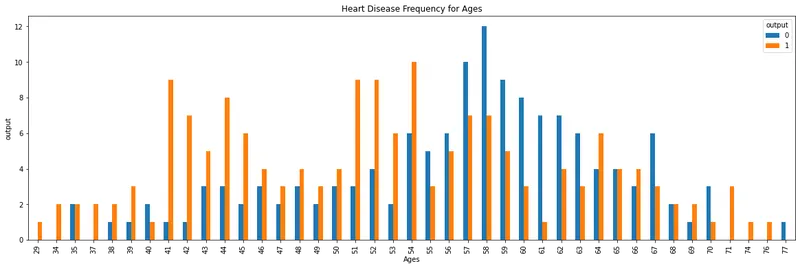
Heart disease Frequency for different aged people

In [97]:

pd.crosstab(data.age,data.output).plot(kind='bar',figsize=(20,6))
plt.title('Heart Disease Frequency for Ages')
plt.xlabel('Ages')
plt.ylabel('output')
plt.show()

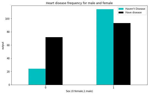
Heart Disease Frequency for male and female

In [139]:

c = ["c","k"]
pd.crosstab(data.sex,data.output).plot(kind='bar',figsize=(10,6),color=c)
plt.title('Heart disease frequency for male and female')
plt.xlabel('Sex (0:female,1:male)')
plt.xticks(rotation=0)
plt.legend(["Haven't Disease", "Have disease "])
plt.ylabel('output')
plt.show()

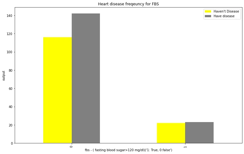
Heart disease frequency based on FBS(Fasting Blood Sugar)

In [120]:

c=["yellow","grey"]
pd.crosstab(data.fbs,data.output).plot(kind="bar",figsize=(13,8),color=c)
plt.title('Heart disease freqeuncy for FBS')
plt.legend(["Haven't Disease", "Have disease "])

plt.xlabel("fbs - ( fasting blood sugar>120 mg/dl)('1: True, 0:false')")
plt.ylabel('output')
plt.show()

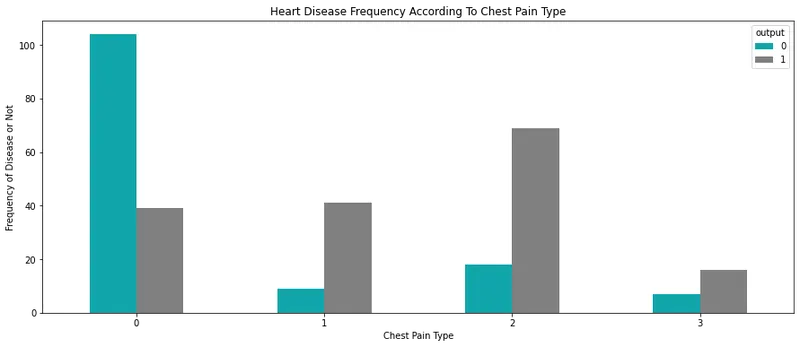
Heart disease frequency according to chest pain type

In [143]:

pd.crosstab(data.cp,data.output).plot(kind="bar",figsize=(15,6),color=['#11A5AA','grey' ])
plt.title('Heart Disease Frequency According To Chest Pain Type')
plt.xlabel('Chest Pain Type')
plt.xticks(rotation = 0)
plt.ylabel('Frequency of Disease or Not')
plt.show()

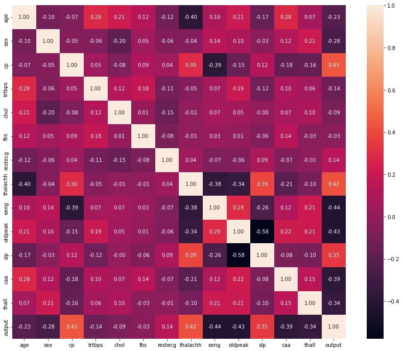
Finding the correlation between the variables

In [125]:

corelation = data.corr()
print(corelation)

               age       sex        cp    trtbps      chol       fbs  \
age       1.000000 -0.098447 -0.068653  0.279351  0.213678  0.121308   
sex      -0.098447  1.000000 -0.049353 -0.056769 -0.197912  0.045032   
cp       -0.068653 -0.049353  1.000000  0.047608 -0.076904  0.094444   
trtbps    0.279351 -0.056769  0.047608  1.000000  0.123174  0.177531   
chol      0.213678 -0.197912 -0.076904  0.123174  1.000000  0.013294   
fbs       0.121308  0.045032  0.094444  0.177531  0.013294  1.000000   
restecg  -0.116211 -0.058196  0.044421 -0.114103 -0.151040 -0.084189   
thalachh -0.398522 -0.044020  0.295762 -0.046698 -0.009940 -0.008567   
exng      0.096801  0.141664 -0.394280  0.067616  0.067023  0.025665   
oldpeak   0.210013  0.096093 -0.149230  0.193216  0.053952  0.005747   
slp      -0.168814 -0.030711  0.119717 -0.121475 -0.004038 -0.059894   
caa       0.276326  0.118261 -0.181053  0.101389  0.070511  0.137979   
thall     0.068001  0.210041 -0.161736  0.062210  0.098803 -0.032019   
output   -0.225439 -0.280937  0.433798 -0.144931 -0.085239 -0.028046   

           restecg  thalachh      exng   oldpeak       slp       caa  \
age      -0.116211 -0.398522  0.096801  0.210013 -0.168814  0.276326   
sex      -0.058196 -0.044020  0.141664  0.096093 -0.030711  0.118261   
cp        0.044421  0.295762 -0.394280 -0.149230  0.119717 -0.181053   
trtbps   -0.114103 -0.046698  0.067616  0.193216 -0.121475  0.101389   
chol     -0.151040 -0.009940  0.067023  0.053952 -0.004038  0.070511   
fbs      -0.084189 -0.008567  0.025665  0.005747 -0.059894  0.137979   
restecg   1.000000  0.044123 -0.070733 -0.058770  0.093045 -0.072042   
thalachh  0.044123  1.000000 -0.378812 -0.344187  0.386784 -0.213177   
exng     -0.070733 -0.378812  1.000000  0.288223 -0.257748  0.115739   
oldpeak  -0.058770 -0.344187  0.288223  1.000000 -0.577537  0.222682   
slp       0.093045  0.386784 -0.257748 -0.577537  1.000000 -0.080155   
caa      -0.072042 -0.213177  0.115739  0.222682 -0.080155  1.000000   
thall    -0.011981 -0.096439  0.206754  0.210244 -0.104764  0.151832   
output    0.137230  0.421741 -0.436757 -0.430696  0.345877 -0.391724   

             thall    output  
age       0.068001 -0.225439  
sex       0.210041 -0.280937  
cp       -0.161736  0.433798  
trtbps    0.062210 -0.144931  
chol      0.098803 -0.085239  
fbs      -0.032019 -0.028046  
restecg  -0.011981  0.137230  
thalachh -0.096439  0.421741  
exng      0.206754 -0.436757  
oldpeak   0.210244 -0.430696  
slp      -0.104764  0.345877  
caa       0.151832 -0.391724  
thall     1.000000 -0.344029  
output   -0.344029  1.000000

Heatmap

In [131]:

plt.figure(figsize=(15,12))
heat = sns.heatmap(corelation,square=True,annot=True,fmt='.2f')
heat.set_xticklabels(heat.get_xticklabels(),rotation=0)
plt.show()

Creating dummies for categorical columns

In [145]:

a = pd.get_dummies(data['cp'],prefix='cp')
b = pd.get_dummies(data['thall'],prefix = 'thal')
c = pd.get_dummies(data['slp'],prefix = 'slp')

In [146]:

frames = [data,a,b,c]
data = pd.concat(frames,axis=1)
data.head()

Out[146]:

	age	sex	cp	trtbps	chol	fbs	restecg	thalachh	exng	oldpeak	...	cp_1	cp_2	cp_3	thal_1	thal_2	slp_0	slp_2
0	63	1	3	145	233	1	0	150	0	2.3	...	0	0	1	1	0	1	0
1	37	1	2	130	250	0	1	187	0	3.5	...	0	1	0	0	1	1	0
2	41	0	1	130	204	0	0	172	0	1.4	...	1	0	0	0	1	0	1
3	56	1	1	120	236	0	1	178	0	0.8	...	1	0	0	0	1	0	1
4	57	0	0	120	354	0	1	163	1	0.6	...	0	0	0	0	1	0	1

5 rows × 25 columns

Removing the categorical columns as we created dummies for those columns

In [148]:

data=data.drop(columns= ['cp','thall','slp'])

In [150]:

data.head()

Out[150]:

	age	sex	trtbps	chol	fbs	restecg	thalachh	exng	oldpeak	...	cp_1	cp_2	cp_3	thal_1	thal_2	slp_0	slp_2
0	63	1	145	233	1	0	150	0	2.3	...	0	0	1	1	0	1	0
1	37	1	130	250	0	1	187	0	3.5	...	0	1	0	0	1	1	0
2	41	0	130	204	0	0	172	0	1.4	...	1	0	0	0	1	0	1
3	56	1	120	236	0	1	178	0	0.8	...	1	0	0	0	1	0	1
4	57	0	120	354	0	1	163	1	0.6	...	0	0	0	0	1	0	1

5 rows × 22 columns

Normalising the data

In [151]:

y = data.output.values
x_data = data.drop(['output'],axis=1)

In [153]:

 x = (x_data - np.min(x_data))/ (np.max(x_data)-np.min(x_data))

C:\anaconda\lib\site-packages\numpy\core\fromnumeric.py:84: FutureWarning: In a future version, DataFrame.min(axis=None) will return a scalar min over the entire DataFrame. To retain the old behavior, use 'frame.min(axis=0)' or just 'frame.min()'
  return reduction(axis=axis, out=out, **passkwargs)
C:\anaconda\lib\site-packages\numpy\core\fromnumeric.py:84: FutureWarning: In a future version, DataFrame.max(axis=None) will return a scalar max over the entire DataFrame. To retain the old behavior, use 'frame.max(axis=0)' or just 'frame.max()'
  return reduction(axis=axis, out=out, **passkwargs)
C:\anaconda\lib\site-packages\numpy\core\fromnumeric.py:84: FutureWarning: In a future version, DataFrame.min(axis=None) will return a scalar min over the entire DataFrame. To retain the old behavior, use 'frame.min(axis=0)' or just 'frame.min()'
  return reduction(axis=axis, out=out, **passkwargs)

Train-Test-split

In [154]:

train_x,test_x,train_y,test_y = train_test_split(x,y,test_size=0.3,random_state=1)

Logistic Regression

In [163]:

accuracies ={}
lr = LogisticRegression()
lr.fit(train_x,train_y)

accur = lr.score(test_x,test_y)*100

accuracies['Logistic Regression '] = accur

print("Accuracy score of Logistic regression Model : {:.2f} %".format(accur))

Accuracy score of Logistic regression Model : 81.32 %

Logistic Regression Model works with 81.32% accuracy

K-Nearest Neighbour (KNN) Classification

In [168]:

knn = KNeighborsClassifier(n_neighbors=2)
knn.fit(train_x,train_y)
prediction = knn.predict(test_x)

print(" Nearest-Neighbor Accuracy Score for n = {} neighbors: {:.2f} %".format(2,knn.score(test_x,test_y)*100))

 Nearest-Neighbor Accuracy Score for n = 2 neighbors: 74.73 %

Now to find the N-value to find the best accuracy score that fits the model

In [181]:

scoreList = []

for i in range(1,20):
    knn2 = KNeighborsClassifier(n_neighbors=i)
    knn2.fit(train_x,train_y)
    scoreList.append(knn2.score(test_x,test_y))
    
plt.plot(range(1,20),scoreList)
plt.xticks(np.arange(1,20,1))
plt.xlabel('K-Value')
plt.ylabel('Score')
plt.show()

# Caluclating highest accuracy for the value of k
accu = max(scoreList)*100
accuracies['KNN'] = accu

print("Maximum accuracy for NN model is {:.2f} % ".format(accu))

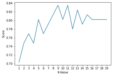
Maximum accuracy for NN model is 83.52 %

As we can see above , for k-value - 9 and 11 , the model has highest accuracy.

KNN Model Accuracy is 83.52%

Support Vector Machine Algorithm

In [188]:

svm = SVC(random_state = 1)
svm.fit(train_x,train_y)
acc = svm.score(test_x,test_y)*100

accuracies['SVM'] = acc

print("SVM accuracy score is : {:.2f} %".format(acc))

SVM accuracy score is : 78.02 %

Decision Tree Classifier

In [190]:

dtc = DecisionTreeClassifier()
dtc.fit(train_x,train_y)

accura = dtc.score(test_x,test_y)*100

accuracies['DecisionTreeClassifier'] = accura

print("Accuracy Score of DecisionTree Classifier is : {:.2f}".format(accura))

Accuracy Score of DecisionTree Classifier is : 71.43

Random Forest Classifier

In [201]:

rfc = RandomForestClassifier(n_estimators=1500,random_state=4)
rfc.fit(train_x,train_y)

accuracy = rfc.score(test_x,test_y)*100

accuracies['RandomForestClassifier']=accuracy

print("Accuracy Score of Random Forest Classifier is : {:.2f} %".format(accuracy))

Accuracy Score of Random Forest Classifier is : 76.92 %

Comparing the Models

In [211]:

colors = ["purple", "green", "orange","#CFC60E","#0FBBAE"]

sns.set_style("whitegrid")
plt.figure(figsize=(12,7))
plt.yticks(np.arange(0,100,10))
plt.xlabel("Algorithms")
plt.ylabel("Accuracy")
sns.barplot(x=list(accuracies.keys()),y=list(accuracies.values()),palette=colors)
plt.show()

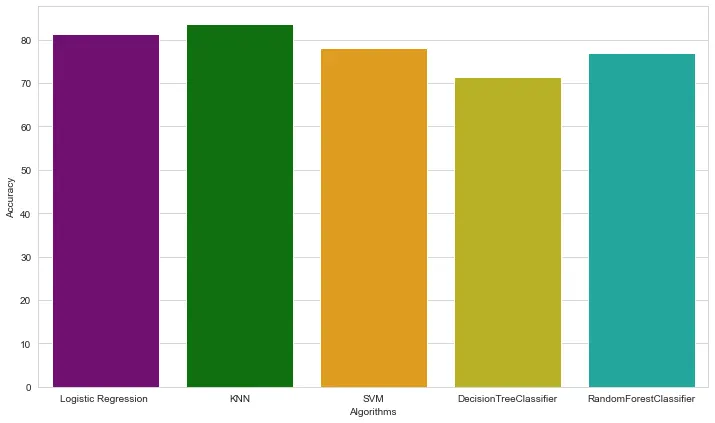
From the above comparison ,

All the models worked well

but the KNN algorithm has the highest accuracy with 83.52%

Now let's look at their confusion matrices

Confusion Matrix

In [213]:

# Predicted Values

y_head_lr = lr.predict(test_x)

knn9 = KNeighborsClassifier(n_neighbors=9)
knn9.fit(train_x,train_y)
y_head_knn = knn9.predict(test_x)

y_head_svm = svm.predict(test_x)

y_head_dtc = dtc.predict(test_x)

y_head_rfc = rfc.predict(test_x)

In [214]:

# Confusion Matrices

cm_lr = confusion_matrix(test_y,y_head_lr)

cm_knn = confusion_matrix(test_y,y_head_knn)

cm_svm = confusion_matrix(test_y,y_head_svm)

cm_dtc = confusion_matrix(test_y,y_head_dtc)

cm_rfc = confusion_matrix(test_y,y_head_rfc)

In [219]:

plt.figure(figsize=(24,12))

plt.suptitle(" Confusion Matrices",fontsize=28)

plt.subplots_adjust(wspace=0.4,hspace=0.4)

plt.subplot(2,3,1)
plt.title("Logistic Regression Confusion Matrix")
sns.heatmap(cm_lr,annot=True,cmap="Blues",fmt="d",cbar=False,annot_kws={"size":28})

plt.subplot(2,3,2)
plt.title("KNN ALgorithm Confusion Matrix ")
sns.heatmap(cm_knn,annot=True,cmap="Blues",fmt="d",cbar=False,annot_kws={"size":24})

plt.subplot(2,3,3)
plt.title("SVM ALgorithm Confusion Matrix")
sns.heatmap(cm_svm,annot=True, cmap="Blues", fmt="d", cbar=False,annot_kws={"size":24})

plt.subplot(2,3,4)
plt.title("Decision Tree Classifier Confusion Matrix")
sns.heatmap(cm_dtc,annot=True , cmap="Blues",fmt = "d", cbar=False,annot_kws={"size":24})

plt.subplot(2,3,5)
plt.title("Random Forest Classifier ConfusionMatrix")
sns.heatmap(cm_rfc,annot=True,cmap="Blues",fmt="d",cbar=False,annot_kws={"size":24})

plt.show()

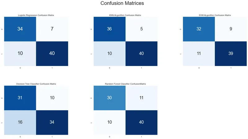
When you working on the health of patients then accuracy is deciding factor,

Applying different machine learning algorithms and checking the accuracy about predictions whether or not the patient has heart disease.

In [ ]:

Thanks & Regards ,

Sai Sumanth Reddy

Project 1

Prediction on getting attacked by Heart Disease

Importing Libraries

Loading Dataset

Heart disease Frequency for different aged people

Heart Disease Frequency for male and female

Heart disease frequency based on FBS(Fasting Blood Sugar)

Heart disease frequency according to chest pain type

Finding the correlation between the variables

Heatmap

Creating dummies for categorical columns

Removing the categorical columns as we created dummies for those columns

Normalising the data

Train-Test-split

Logistic Regression

K-Nearest Neighbour (KNN) Classification

Support Vector Machine Algorithm

Decision Tree Classifier

Random Forest Classifier

Comparing the Models

but the KNN algorithm has the highest accuracy with 83.52%

Confusion Matrix

Ship work like this
in your own course.

Talk to a career counsellor

	age	sex	cp	trtbps	chol	fbs	restecg	thalachh	exng	oldpeak	slp	caa	thall	output
0	63	1	3	145	233	1	0	150	0	2.3	0	0	1	1
1	37	1	2	130	250	0	1	187	0	3.5	0	0	2	1
2	41	0	1	130	204	0	0	172	0	1.4	2	0	2	1
3	56	1	1	120	236	0	1	178	0	0.8	2	0	2	1
4	57	0	0	120	354	0	1	163	1	0.6	2	0	2	1
...	...	...	...	...	...	...	...	...	...	...	...	...	...	...
298	57	0	0	140	241	0	1	123	1	0.2	1	0	3	0
299	45	1	3	110	264	0	1	132	0	1.2	1	0	3	0
300	68	1	0	144	193	1	1	141	0	3.4	1	2	3	0
301	57	1	0	130	131	0	1	115	1	1.2	1	1	3	0
302	57	0	1	130	236	0	0	174	0	0.0	1	1	2	0

	age	sex	cp	trtbps	chol	fbs	restecg	thalachh	exng	oldpeak	slp	thall	output
0	63	1	3	145	233	1	0	150	0	2.3	0	1	1
1	37	1	2	130	250	0	1	187	0	3.5	0	2	1
2	41	0	1	130	204	0	0	172	0	1.4	2	2	1
3	56	1	1	120	236	0	1	178	0	0.8	2	2	1
4	57	0	0	120	354	0	1	163	1	0.6	2	2	1

	age	sex	cp	trtbps	chol	fbs	restecg	thalachh	exng	oldpeak	slp	caa	thall
298	57	0	0	140	241	0	1	123	1	0.2	1	0	3
299	45	1	3	110	264	0	1	132	0	1.2	1	0	3
300	68	1	0	144	193	1	1	141	0	3.4	1	2	3
301	57	1	0	130	131	0	1	115	1	1.2	1	1	3
302	57	0	1	130	236	0	0	174	0	0.0	1	1	2

	age	sex	cp	trtbps	chol	fbs	restecg	thalachh	exng	oldpeak	...	cp_1	cp_2	cp_3	thal_1	thal_2	slp_0	slp_2
0	63	1	3	145	233	1	0	150	0	2.3	...	0	0	1	1	0	1	0
1	37	1	2	130	250	0	1	187	0	3.5	...	0	1	0	0	1	1	0
2	41	0	1	130	204	0	0	172	0	1.4	...	1	0	0	0	1	0	1
3	56	1	1	120	236	0	1	178	0	0.8	...	1	0	0	0	1	0	1
4	57	0	0	120	354	0	1	163	1	0.6	...	0	0	0	0	1	0	1

	age	sex	trtbps	chol	fbs	restecg	thalachh	exng	oldpeak	...	cp_1	cp_2	cp_3	thal_1	thal_2	slp_0	slp_2
0	63	1	145	233	1	0	150	0	2.3	...	0	0	1	1	0	1	0
1	37	1	130	250	0	1	187	0	3.5	...	0	1	0	0	1	1	0
2	41	0	130	204	0	0	172	0	1.4	...	1	0	0	0	1	0	1
3	56	1	120	236	0	1	178	0	0.8	...	1	0	0	0	1	0	1
4	57	0	120	354	0	1	163	1	0.6	...	0	0	0	0	1	0	1

	age	sex	cp	trtbps	chol	fbs	restecg	thalachh	exng	oldpeak	slp	caa	thall	output
0	63	1	3	145	233	1	0	150	0	2.3	0	0	1	1
1	37	1	2	130	250	0	1	187	0	3.5	0	0	2	1
2	41	0	1	130	204	0	0	172	0	1.4	2	0	2	1
3	56	1	1	120	236	0	1	178	0	0.8	2	0	2	1
4	57	0	0	120	354	0	1	163	1	0.6	2	0	2	1
...	...	...	...	...	...	...	...	...	...	...	...	...	...	...
298	57	0	0	140	241	0	1	123	1	0.2	1	0	3	0
299	45	1	3	110	264	0	1	132	0	1.2	1	0	3	0
300	68	1	0	144	193	1	1	141	0	3.4	1	2	3	0
301	57	1	0	130	131	0	1	115	1	1.2	1	1	3	0
302	57	0	1	130	236	0	0	174	0	0.0	1	1	2	0

	age	sex	cp	trtbps	chol	fbs	restecg	thalachh	exng	oldpeak	slp	thall	output
0	63	1	3	145	233	1	0	150	0	2.3	0	1	1
1	37	1	2	130	250	0	1	187	0	3.5	0	2	1
2	41	0	1	130	204	0	0	172	0	1.4	2	2	1
3	56	1	1	120	236	0	1	178	0	0.8	2	2	1
4	57	0	0	120	354	0	1	163	1	0.6	2	2	1

	age	sex	cp	trtbps	chol	fbs	restecg	thalachh	exng	oldpeak	slp	caa	thall
298	57	0	0	140	241	0	1	123	1	0.2	1	0	3
299	45	1	3	110	264	0	1	132	0	1.2	1	0	3
300	68	1	0	144	193	1	1	141	0	3.4	1	2	3
301	57	1	0	130	131	0	1	115	1	1.2	1	1	3
302	57	0	1	130	236	0	0	174	0	0.0	1	1	2

	age	sex	cp	trtbps	chol	fbs	restecg	thalachh	exng	oldpeak	...	cp_1	cp_2	cp_3	thal_1	thal_2	slp_0	slp_2
0	63	1	3	145	233	1	0	150	0	2.3	...	0	0	1	1	0	1	0
1	37	1	2	130	250	0	1	187	0	3.5	...	0	1	0	0	1	1	0
2	41	0	1	130	204	0	0	172	0	1.4	...	1	0	0	0	1	0	1
3	56	1	1	120	236	0	1	178	0	0.8	...	1	0	0	0	1	0	1
4	57	0	0	120	354	0	1	163	1	0.6	...	0	0	0	0	1	0	1

	age	sex	trtbps	chol	fbs	restecg	thalachh	exng	oldpeak	...	cp_1	cp_2	cp_3	thal_1	thal_2	slp_0	slp_2
0	63	1	145	233	1	0	150	0	2.3	...	0	0	1	1	0	1	0
1	37	1	130	250	0	1	187	0	3.5	...	0	1	0	0	1	1	0
2	41	0	130	204	0	0	172	0	1.4	...	1	0	0	0	1	0	1
3	56	1	120	236	0	1	178	0	0.8	...	1	0	0	0	1	0	1
4	57	0	120	354	0	1	163	1	0.6	...	0	0	0	0	1	0	1

Prediction on getting attacked by Heart Disease

Importing Libraries

Loading Dataset

Heart disease Frequency for different aged people

Heart Disease Frequency for male and female

Heart disease frequency based on FBS(Fasting Blood Sugar)

Heart disease frequency according to chest pain type

Finding the correlation between the variables

Heatmap

Creating dummies for categorical columns

Removing the categorical columns as we created dummies for those columns

Normalising the data

Train-Test-split

Logistic Regression

K-Nearest Neighbour (KNN) Classification

Support Vector Machine Algorithm

Decision Tree Classifier

Random Forest Classifier

Comparing the Models

but the KNN algorithm has the highest accuracy with 83.52%

Confusion Matrix

Ship work like thisin your own course.

Talk to a career counsellor

Ship work like this
in your own course.

	age	sex	cp	trtbps	chol	fbs	restecg	thalachh	exng	oldpeak	slp	caa	thall	output
0	63	1	3	145	233	1	0	150	0	2.3	0	0	1	1
1	37	1	2	130	250	0	1	187	0	3.5	0	0	2	1
2	41	0	1	130	204	0	0	172	0	1.4	2	0	2	1
3	56	1	1	120	236	0	1	178	0	0.8	2	0	2	1
4	57	0	0	120	354	0	1	163	1	0.6	2	0	2	1
...	...	...	...	...	...	...	...	...	...	...	...	...	...	...
298	57	0	0	140	241	0	1	123	1	0.2	1	0	3	0
299	45	1	3	110	264	0	1	132	0	1.2	1	0	3	0
300	68	1	0	144	193	1	1	141	0	3.4	1	2	3	0
301	57	1	0	130	131	0	1	115	1	1.2	1	1	3	0
302	57	0	1	130	236	0	0	174	0	0.0	1	1	2	0

	age	sex	cp	trtbps	chol	fbs	restecg	thalachh	exng	oldpeak	slp	thall	output
0	63	1	3	145	233	1	0	150	0	2.3	0	1	1
1	37	1	2	130	250	0	1	187	0	3.5	0	2	1
2	41	0	1	130	204	0	0	172	0	1.4	2	2	1
3	56	1	1	120	236	0	1	178	0	0.8	2	2	1
4	57	0	0	120	354	0	1	163	1	0.6	2	2	1

	age	sex	cp	trtbps	chol	fbs	restecg	thalachh	exng	oldpeak	slp	caa	thall
298	57	0	0	140	241	0	1	123	1	0.2	1	0	3
299	45	1	3	110	264	0	1	132	0	1.2	1	0	3
300	68	1	0	144	193	1	1	141	0	3.4	1	2	3
301	57	1	0	130	131	0	1	115	1	1.2	1	1	3
302	57	0	1	130	236	0	0	174	0	0.0	1	1	2

	age	sex	cp	trtbps	chol	fbs	restecg	thalachh	exng	oldpeak	...	cp_1	cp_2	cp_3	thal_1	thal_2	slp_0	slp_2
0	63	1	3	145	233	1	0	150	0	2.3	...	0	0	1	1	0	1	0
1	37	1	2	130	250	0	1	187	0	3.5	...	0	1	0	0	1	1	0
2	41	0	1	130	204	0	0	172	0	1.4	...	1	0	0	0	1	0	1
3	56	1	1	120	236	0	1	178	0	0.8	...	1	0	0	0	1	0	1
4	57	0	0	120	354	0	1	163	1	0.6	...	0	0	0	0	1	0	1

	age	sex	trtbps	chol	fbs	restecg	thalachh	exng	oldpeak	...	cp_1	cp_2	cp_3	thal_1	thal_2	slp_0	slp_2
0	63	1	145	233	1	0	150	0	2.3	...	0	0	1	1	0	1	0
1	37	1	130	250	0	1	187	0	3.5	...	0	1	0	0	1	1	0
2	41	0	130	204	0	0	172	0	1.4	...	1	0	0	0	1	0	1
3	56	1	120	236	0	1	178	0	0.8	...	1	0	0	0	1	0	1
4	57	0	120	354	0	1	163	1	0.6	...	0	0	0	0	1	0	1