Project 1
Title: Development of a forward energy-based fuel consumption model for a conventional vehicle.
Aim of project:
1] Build Simulink model using blocks and complete the vehicle model.
2] Writting scripts in MATLAB to load all the variables required for running the Simulink model.
3] Tabulate the fuel economy numbers (kmpl) for UDDS and HWFET cycle.
4] Plot the time trace for engine, transmission input, transmission output and wheel speed on one plot.
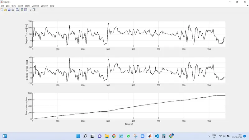
5] Plot engine torque, engine power, fuel rate and fuel consumption using subplots.
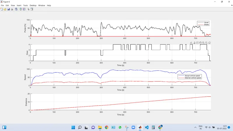
6] Plot accelerator and brake pedal, gear command, vehicle desired and actual speed, vehicle distance using subplots.
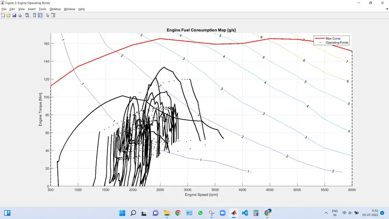
7] Plot the engine operating points on the engine fuel map.
8] Generate the plots for both drive cycles.
9] Study of Conventional vehicle simulink model and creates graphs.
A forward energy-based model is one in which the transmission torque at a particular instant of time is the power demand at the wheels.
A conventional vehicle is an ic engine that relies on gasoline or diesel as its power source.
Matlab code:
It consists of two files:
Initialization script: it consists of defining all the variables used in the Simulink model and is thus necessary for running the script before running the Simulink model.
running the initialization file defines all the variables in the workspace which will be useful in running the simulation.
Initialization script in Matlab:
%%%%%%%%%%%%%%%%%%%%%%%%%%%%%%%%%%%%%%%%%%%%%%%%%%%%%%%%%%%%%%%%%%%%%
%% Skill-Lync -> Hybrid Drives Development
% Project 1 - Conventional Vehicle Model
% By - Ullekh Gambhira

% Description:

%% Initialization File
% Initialization file for loading the variables for the Conventional vehicle simulation model

%% Vehicle Parameters
M = 1500;       % Vehicle weight [kg]
Cr = 0.015;     % Rolling resistance coefficient
Rw = 0.35;      % Rolling radius [m]
Cd = 0.33;      % Drag coefficient
Af = 2;         % Frontal area [m2]
rhoa = 1.225;   % Air density [kg/m3]
Vwind = 0;      % Wind velocity [kmph]
g = 9.81;       % Gravitational acceleration [m/s2]
theta = 0;      % Slope [deg]
myu_road_tire = 1; % Coefficient of friction between tire - road interface

%% Powertrain Parameters
FDR = 3.73;                         % Final Drive Ratio / Diff Ratio
DiffEff = 0.99;                     % Differential efficiency (assumed independent of operating conditions)

NumGear = 4;                        % Number of gears in transmission
TransGear = [1:NumGear];            % Transmission Gears
TransRatio = [3.06, 1.62, 1, 0.7];  % Corresponding Transmission ratios
TransEff = 0.90;                    % Transmission efficiency (assumed independent of operating conditions)

TC_SR = [0, .5, .6, .7, .8, .87, .92, .94, .96, .97, 1];   % Torque Converter Speed Ratio (Matlab default) -> TurbSpd/PumpSpd
TC_TR = [2.232, 1.5462, 1.4058, 1.2746, 1.1528, 1.0732, 1.0192, 1, 1, 1, 1];   % Torque Converter Torque Ratio (Matlab default) -> TurbTrq/PumpTrq
TC_Cf = 1e-4 * [.72558, .66322, .63463, .59042, .51331, .4144, .29287, .22444, .12186, .04386, 0]; % Torque Converter Capacity Factor (Matlab default) -> PumpTrq/PumpSpd^2 [Nm/rpm^2]

load Vehicle_Data/Engine_data_1_9L_Saturn_95kW
load Vehicle_Data/Trans_Shift_map

%% Driver Parameters
Kp = 10;                    % P gain for driver PI model
Ki = 1;                     % I gain for driver PI model
Drive_Cycle_Select = 3;     % Drive cycle selection

% Drive cycle values in m/s

if Drive_Cycle_Select == 1
    load DriveCycles/UDDS;

elseif Drive_Cycle_Select == 2
    load DriveCycles/HWFET;

elseif Drive_Cycle_Select == 3
    load DriveCycles/FTP;

elseif Drive_Cycle_Select == 4
    load DriveCycles/US06;

elseif Drive_Cycle_Select == 5
    load DriveCycles/NEDC;

elseif Drive_Cycle_Select == 6
    load DriveCycles/WLTP;

end

time_end = cyc_time(end);
vel_end = cyc_vel(end);
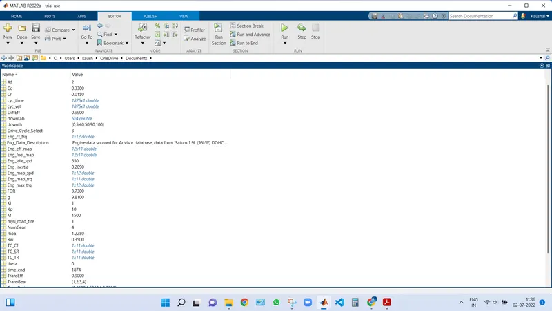
After running the above code all the variables are defined in the workspace as shown below:
Now we can open the project 1 file in the simulink and run it:
The simulink model of the vehicle is as follows:
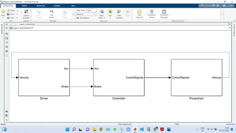
The simulink model consist of three sub systems namely Driver model, Controller block and Power train block.
Driver model:
The input to the driver block is the instantaneous vehicle speed which is compared with the drive cycle speed at that particular instant using the p-i controller logic and the output is brake pedal and accelerator pedal depending on the requirement.
Simulink model of the driver model:
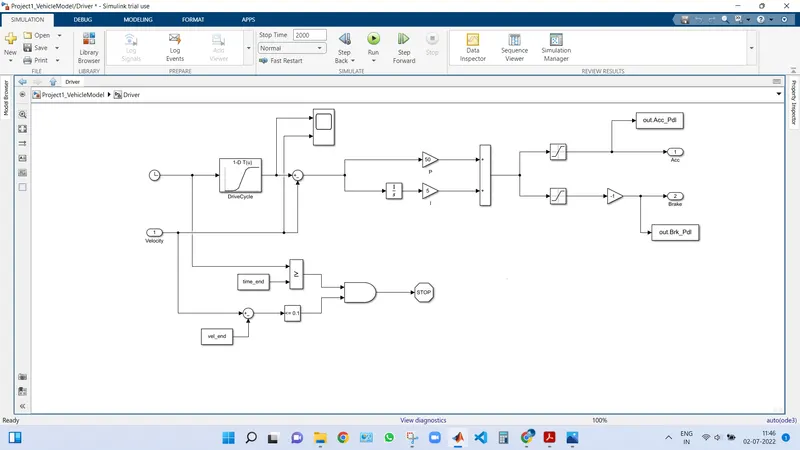
In the Simulink model, we have added an additional To Workspace block in order to send the simulation data directly to the Matlab workspace.
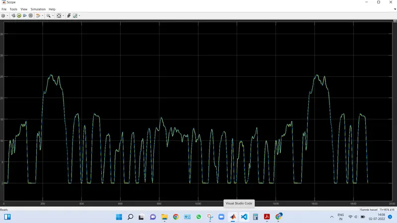
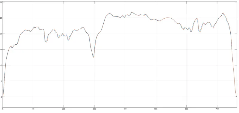
Output from the scope connected to the driver model:
For UDDS cycle
For HWFET cycle
Controller block.
The ‘Controller’ block is the brain of the vehicle, representing the electronic control unit. It is based on the driver inputs, it generates desired engine torque, desired transmission gear, and desired brake torque. These inputs are fed to the ‘Powertrain’ block which represents the drivetrain of the vehicle.
Simulink model of the controller block:
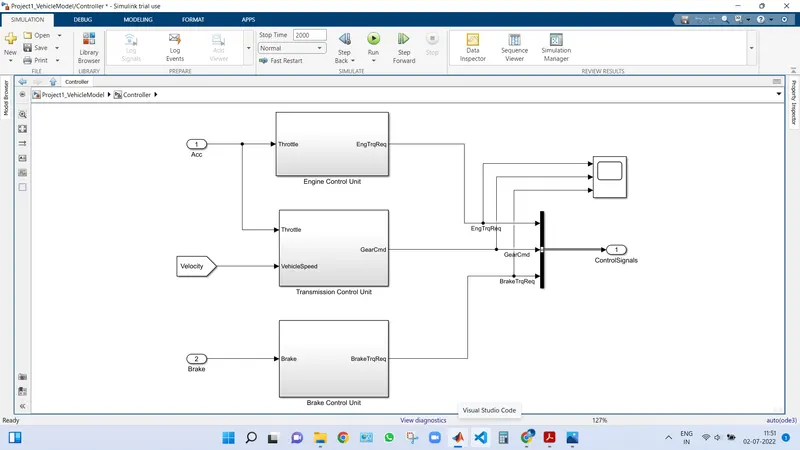
The controller block consists of three subsystem blocks namely the engine control unit, transmission control unit, and brake control unit.
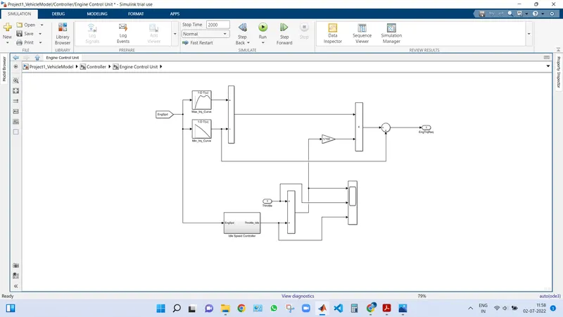
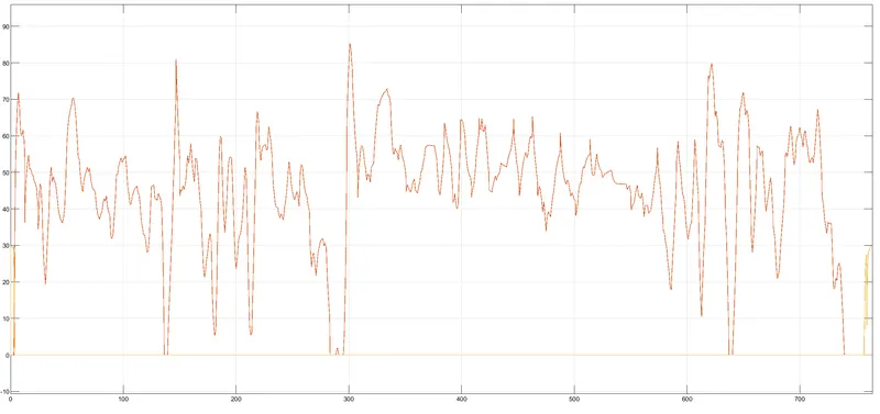
Engine control unit: here the engine torque requirement is calculated using the engine speed and throttle output from the driver block.
Simulink model:
Scope output :
For UDDS cycle
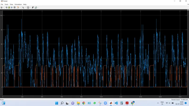
For HWFET cycle
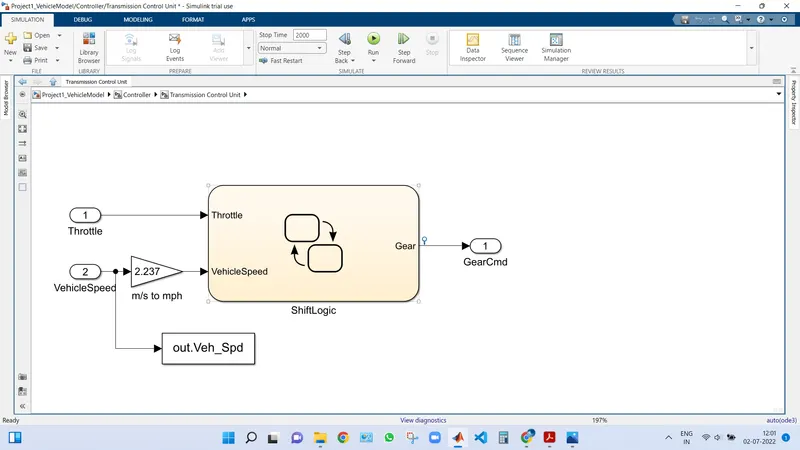
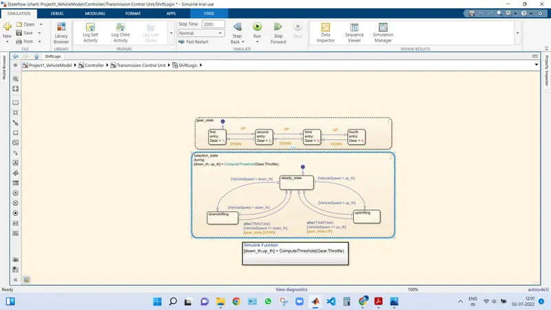
Transmission control unit: Here based on the throttle input from the driver block and comparing it with the actual current vehicle speed appropriate gear is selected and is an input to the transmission block.
Simulink model:
Shift logic:
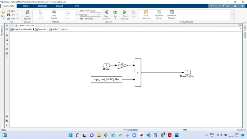
Brake control unit:
In this block the brake torque requirement is calculated.
Simulink model:
Hence the three outputs are engine torque desired transmission gear and desired brake torque using the above controller unit.
Scope output of the controller signals:
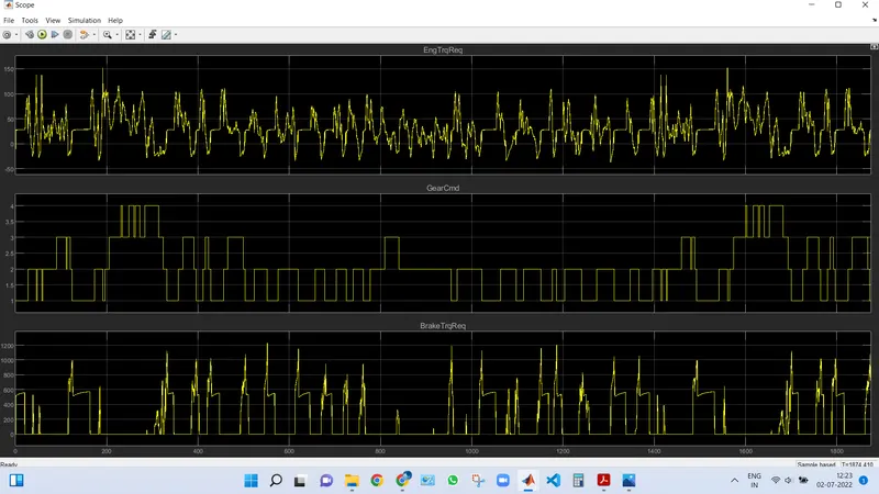
For hwfet cycle
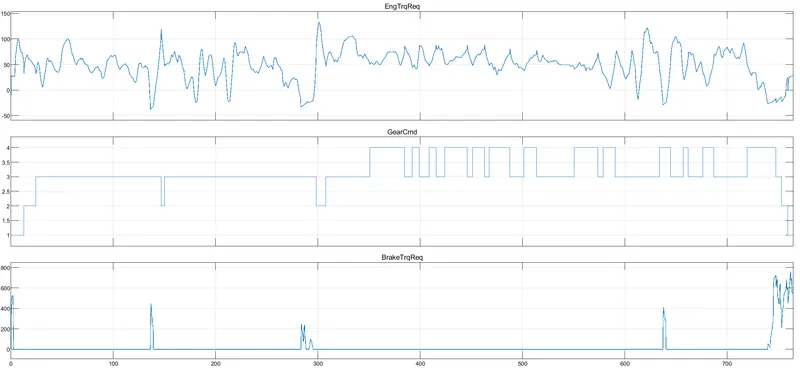
The above plot shows the engine required trq, gear cmd, brake trq req at the various instants of time.
Power train block:
The power train block consists of five subsystems namely:
- Engine block
- transmission block
- differential block
- wheels block and
- vehicle dynamics block
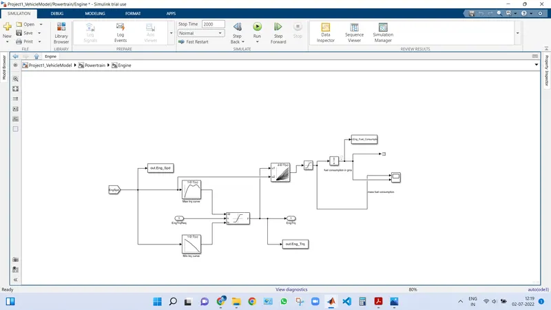
Engine block:
Simulink model:
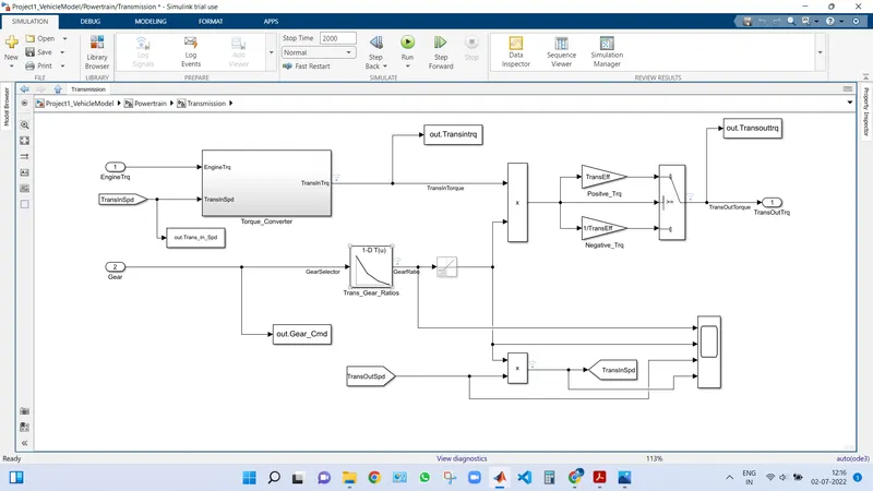
Transmission block:
Simulink model:
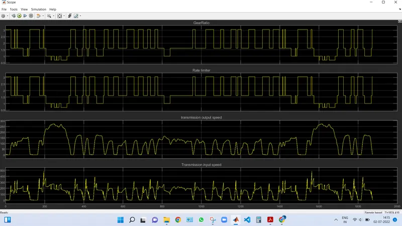
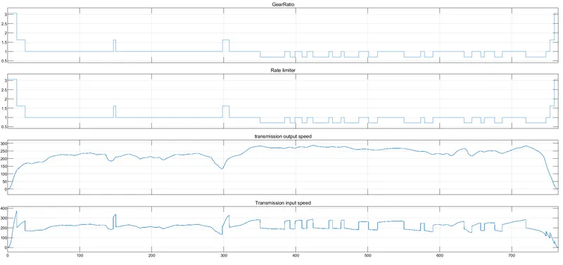
Scope output:
for UDDS CYCLE
For HWFET CYCLE
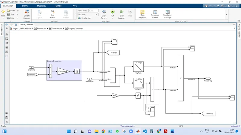
Inside the torque converter block:
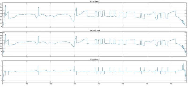
Scope output:
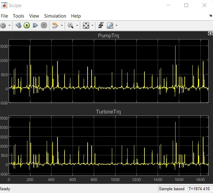
Plot of pump speed turbine speed and speed ratio for hwfet cycle:
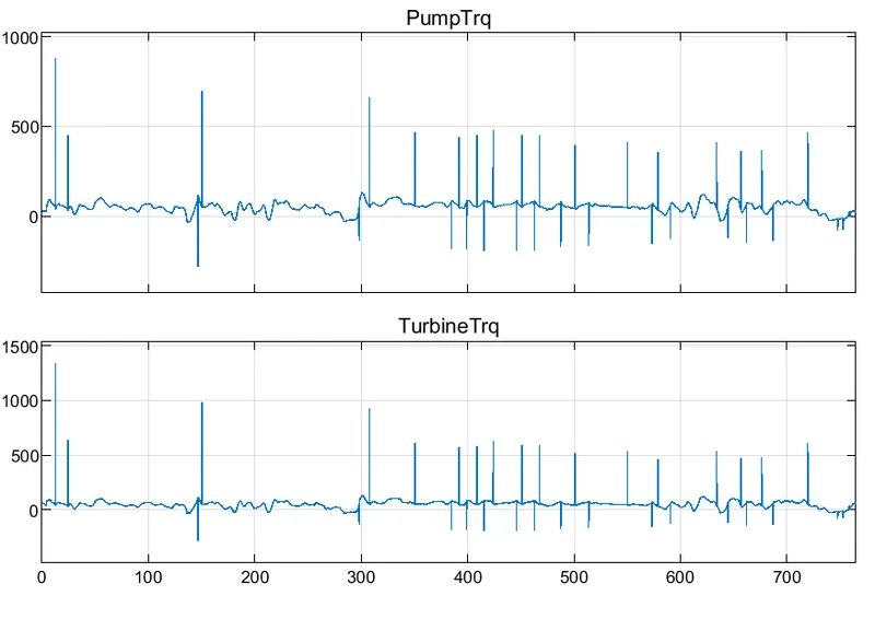
Plot of pump torque and turbine torque:
For hwfet cycle
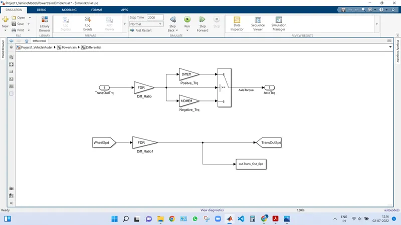
Differential block:
Simulink model:
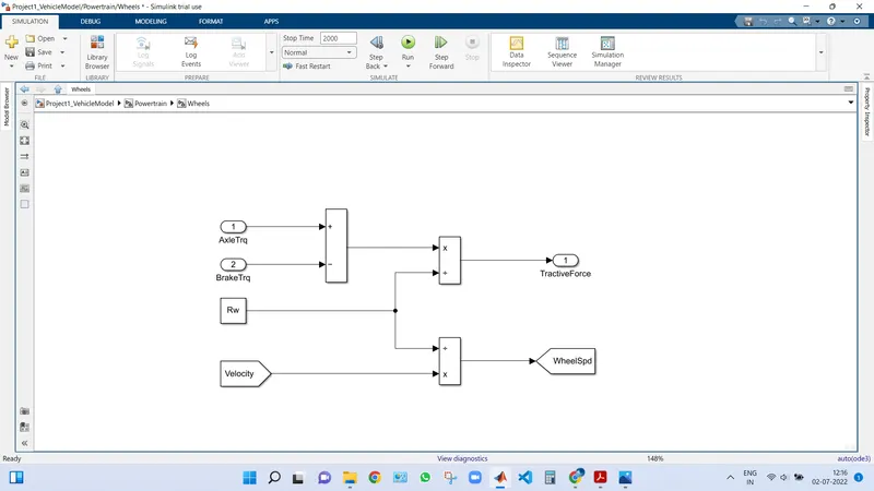
wheels block:
Simulink model:
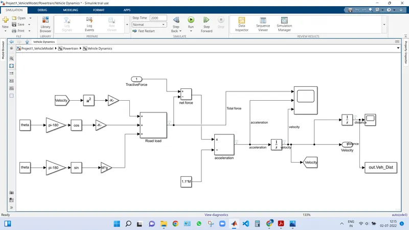
Vehicle dynamics block:
Simulink model:
Scope output:
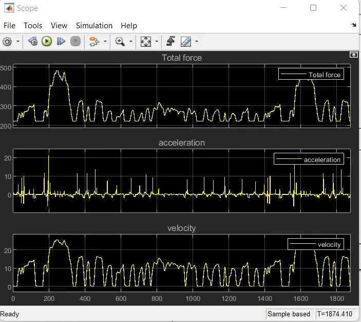
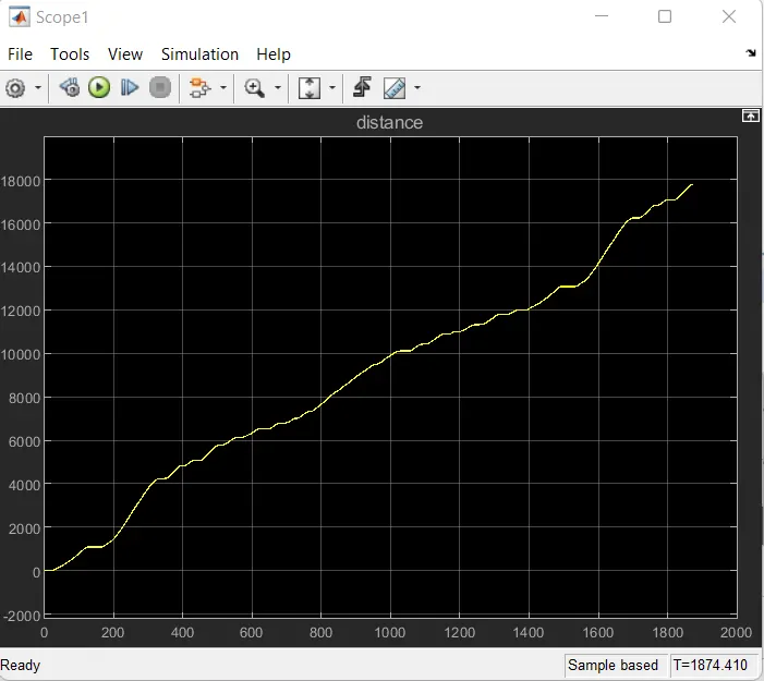
For UDDS cycle:
a. Tabulate the fuel economy numbers (kmpl) for UDDS cycle.
fuel economy numbers (kmpl) for UDDS cycle is =13.6312 kmpl.
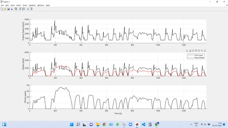
b. Plot the time trace for engine, transmission input, transmission output and wheel speed on one plot.
c. Plot engine torque, engine power, fuel rate and fuel consumption using subplots.
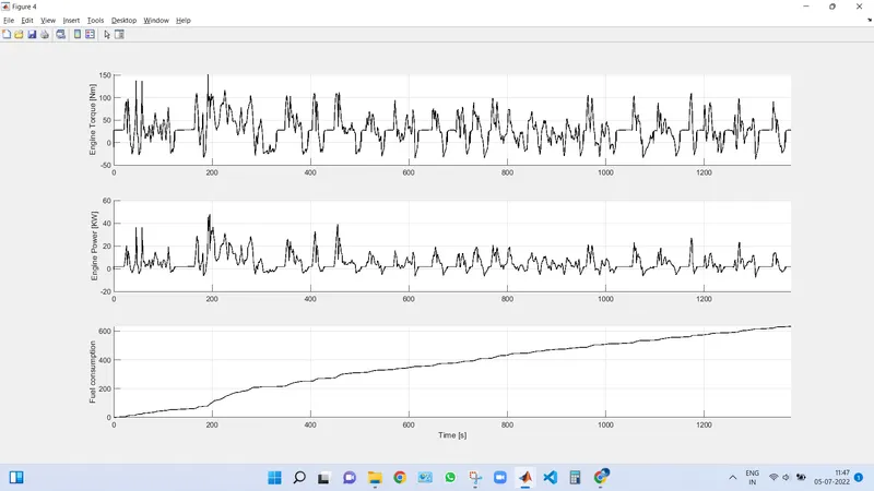
d. Plot accelerator and brake pedal, gear command, vehicle desired and actual speed, vehicle distance using subplots.
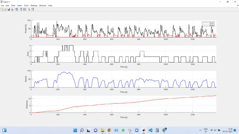
e. Plot the engine operating points on the engine fuel map.
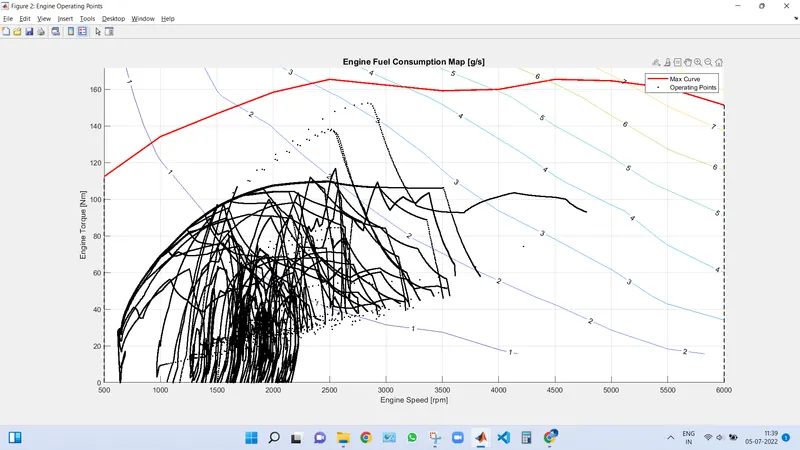
For HWFET cycle:
a. Tabulate the fuel economy numbers (kmpl) for HWFET cycle.
fuel economy numbers (kmpl) for HWFET cycle is 16.3072 kmpl.
b. Plot the time trace for engine, transmission input, transmission output and wheel speed on one plot.
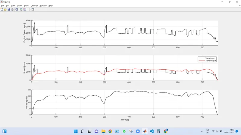
c. Plot engine torque, engine power, fuel rate and fuel consumption using subplots.
d. Plot accelerator and brake pedal, gear command, vehicle desired and actual speed, vehicle distance using subplots.
e. Plot the engine operating points on the engine fuel map.
Tabulate fuel economy for both udds and hwfet cycle:
| CYCLE | Fuel economy (kmpl) |
| UDDS CYCLE | 13.6312 |
| HWFET CYCLE | 16.3072 |