Project 1
Question 1
Objective: In this project we are going to clean the dataset of 1985 automobile dataset.
About the dataset:
This is a raw dataset about cars in 1985.
This dataset set consists of three types of entities:
a the specification of an auto in terms of various characteristics
b its assigned insurance risk rating
c its normalized losses in use as compared to other cars. The second rating corresponds to the degree to which the auto is more risky than its price indicates. Cars are initially assigned a risk factor symbol assosicated with its price. Then, if it is more risky (or less), this symbol is adjusted by moving it up (or down) the scale. Actuarians call this process symboling. A value of +3 indicates that the auto is risky, -3 that it is probably pretty safe. The third factor is the relative average loss payment per insured vehicle year. This value is normalized for all autos within a particular size classification (two-dooe small, station wagons, sports/specialty, etc...), and represents the average loss per car per year.
Note: Several to the attributes in the database could be used as a class attribute.
Number of instances: 205
Number of Attributes: 26 total
-- 15 continous
-- 1 integer
-- 10 nominal.
Attribute Information:
1. Symboling: -3,-2,-1,0,1,2,3
2. normalized-losses: continous from 65 to 256
3. Make: alfa- romero,audi,bmw,chevrolet,dodge,honda,isuzu,jaguar, mazda, mercedes-benz,mercury, mitsubishi, nissan,peugot,plymouth,porshe,renault,saab,subaru,toyota,volkswagen,volvo
4. fuel-type: diesel,gas
5. aspiration: std,turbo
6. num-of-doors: four,two
7. body-style: hardtop,wagon, sedan,hatchback,convertible
8. drive-wheels: 4wd,fwd,rwd
9. engine-location: front, rear
10. wheel-base: continous from 86.6.120.9
11. length: continous from 141.1 to 208.1
12. width: continous from 60.3 to 72.3
13. height: continous from 47.8 to 59.8
14. Curb-weight: continous from 1488 to 4066
15. engine-type: dohc,dohcv,|, ohc, ohcf,ohcc,rotor
16. num-of-cylinders: eight,five,four,six,three,twelve,two
17. engine-size:continous from 61 to 326
18. fuel-system: 1bbl,2bbl,4bbl,idi,mfi,mpfi,spdi,spfi
19. bore: continous from 2.54 to 3.94
20. stroke: continous from 2.07 to 4.17
21. compression-ratio: continous from 7 to 23
22. horse power: continous from 48-288
23. peak-rpm: continous from 4150 to 6600
24. city-mpg: continous from 13 to 49
25. highway-mpg: continous from 16 to 54
26. price: continous from 5118 to 45400.
overview:
* Importing the necessary libraries and the raw data.
* renaming the columns.
* Finding the missing values.
* Filling the missing values.
* Exporting the data into a new csvfile.
* summary and conclusion.
1. Importing the necessary libraries and the raw data.
* In the first step, we are going to import the libraries like pandas, nummpy and matplotlib. After that we are going to import the csv file called auto.csv
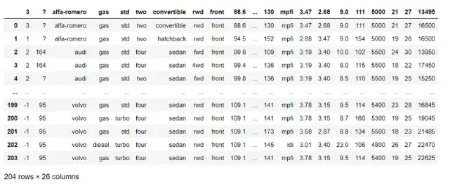
* As we can see that there are 204 data points and 26 attributes in the dataset but the column names are absurdly written. Lets see all the columns at once so that we can get the idea on the number of absurdly written columns.
* By observing the above data we can find that all the column names are absurdly written. So in the next step we will be renaming the columns.
2. Renaming the columns:
* In this step we will first pass a variable named 'column' which contains the array of the new column names and then we will pass this variable to the pandas dataframe to replace it with the new columns names.
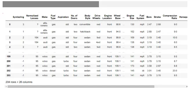
* so in this way we have replaced the new column names with old one.
3. Finding the missing values:
* If we closely look at the data we will find that there are several '?' sign on the data points which indicates that there are some missing values in the dataset.
* As it is difficult to deal with '?' in that dataset we will replacing it with NaN value so that we can easily deal with the null values.
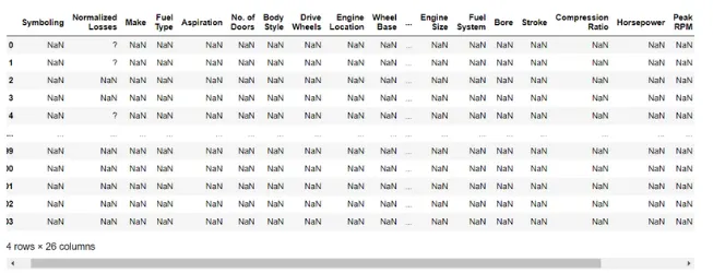
* The replacement of '?' sign to null values is successfully changed.
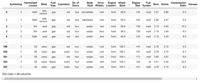
* Now we can easily determine the columns containing the null values.
* By observing the above results we have successfully counted the number missing values in different columns.
According to the results:
1. Normalized losses has 40 missing values.
2. No. of Doors has 2 missing values.
3. Bore has 4 missing values.
4. Stroke has 4 missing values.
5. Horsepower and peak RPM have 2 missing values each.
6. Price has 4 missing values.
* We are now going to check for the number of rows having at atleast one missing values.
For this process, we will first find the indexes of the datasets which contains at least one null values and then pass it on to the dataframe.
These are the indexes of the dataset having at least one missing value throughout the datapoint.
Now we are going to locate all these datapoints at once and counting it.
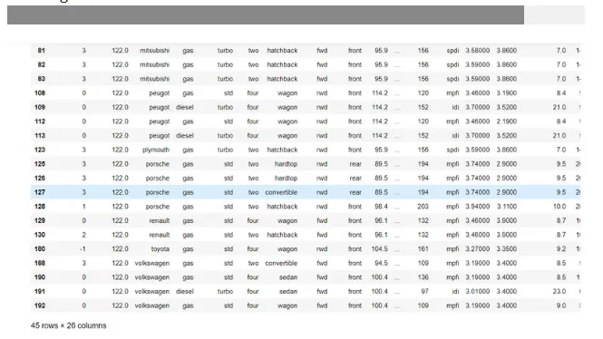
So its been founded out that there are 45 datapoints exist which has at least one missing value.
* Now we are going to check if there is any roww or column having all null values.
So there is no column or row exist which has all the null values.
* Now lets find out the % of the missing values in all the columns.
According to the results it has been found that:
1. Normalized losses is the column having the most null values of about 19.61%.
2. Price, stroke and Bore are the columns containing 1.96% null values each.
3. Peak RPM, Horsepower and No of Doors are the columns containing 0.98% null values each.
4. Filling the missing values:
Now that we know every detail about the missing values in the dataset we will now fill the null values.
We will replace the null values with the mean of the values of that particular column.
In order to do that, the data type of the particular columns should be in floating types, otherwise we will not be able to find the mean of that particular column.
* Changing the data types of that target columns.
Here out target columns are 'Normalized Losses', Price, Stroke, Bore, Peak RPM, Horsepower and No. of Doors. As 'No. of Doors columns is a categorial data it can't be change into float data type. We will deal with this column later.
First we will change the datatype of the target columns excluding 'No. of doors'.
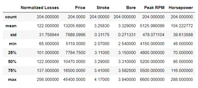
So it is clear that we can find out the mean of the each target columns.
* Replacing the null values in 'Normalized Losses' column with the mean of the column i.e, 122.
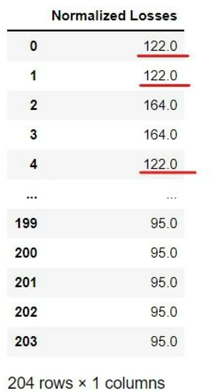
Let us deal with the normalized Losses column first as it contains the most number of null values. We will replace the null values with its mean which is 122.
It looks like all the null values are replaced with the mean value of the column.
Let's check whether actually all the null values are gone or not.
It is clear from the above results that there is no null value left in the Normalized Losses column.
* Similarly performing the same procedure with the rest of the target columns.
We will apply the same method for filling the null values as we did in the previous step.
The null values have been filled successfully except in No. of Doors column.
* Filling the null values in 'No. of Doors' columns.
In this case the data the data is categorial so we first need to look at the data finding the unique values of it.
So it is clear from the above results that there are two unique values under which the column is classified.
As it is a categorial data the 'mean' method won't work here. In this case we need to count the number of these categorial indicators. The indicator which has more number of counts will be used in filling the null value.
The above result indicates that there are more number of cars having four doors than two doors. So, accordingly we will use the four indicator to fill the null values.
We have successfully removed all the null values and hence we have cleaned our whole dataset in this way.
5. Exporting the cleaning dataframe to a csv file:
* The raw data was imported.
* All the columns was renamed.
* The null values was counted.
* All the null values was replaced by the column's mean value.
* In the 'No. of Doors' column the null values are replaced by the most numbered categorial indicator.
* The new dataframe is exported to a csv file.
* Hence the 1985 Automobile Dataset is cleaned.