Project 1
Project 1 deals with the development of a forward energy-based fuel consumption model of a conventional vehicle.
The main goal of this project is to get familiar with the modeling process, writing scripts in Matlab, modeling in Simulink, analyzing data and generating plots.
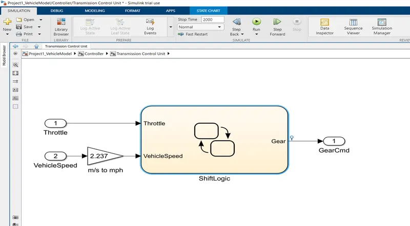
In this project, a typical midsize car with a 1.9L engine and a 4-speed automatic transmission is considered. Data is taken from ADVISOR data base developed by NREL, USA. Transmission shift map and controller is taken from Matlab/Simulink example database.
The model developed has the capability to simulate the vehicle on different drive cycles like UDDS, HWFET, FTP, NEDC, etc.
“Project1_InitFile.m” is a Matlab script used to load all the variables required for running the Simulink model and for post-processing. The drive cycle selection is also done here. Before running the Simulink
vehicle model, run this initialization script.
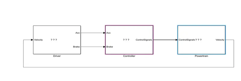
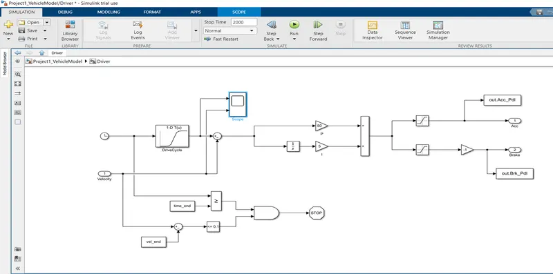
“Project1_VehicleModel.slx” is the Simulink model of the vehicle. It is modeled using a ‘Driver’ block, which is a basic PI controller that generates accelerator and brake pedal outputs to match the desired
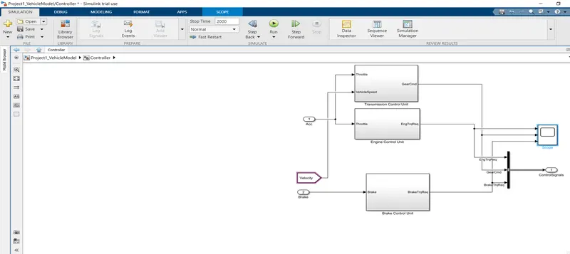
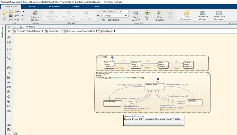
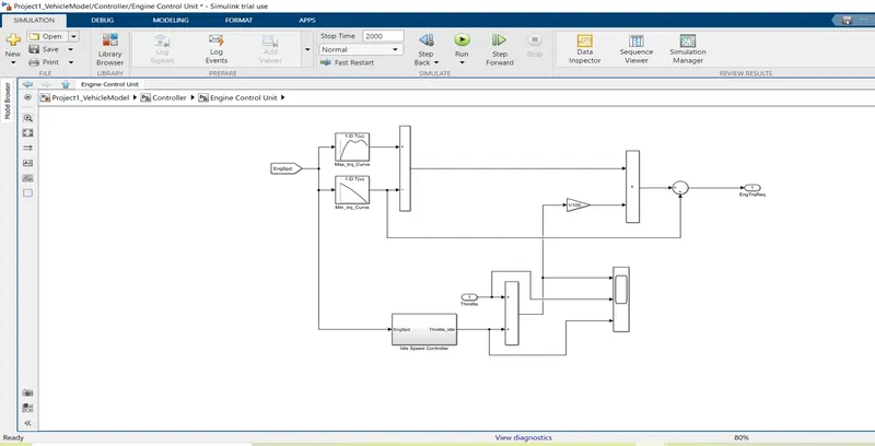
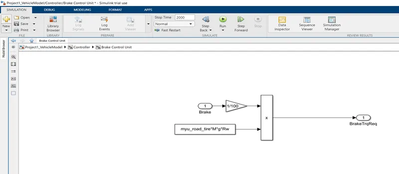
and actual vehicle speeds. The ‘Controller’ block is the brains of the vehicle, representing the electronic controls units. Based on the driver inputs, it generates desired engine torque, desired transmission gear
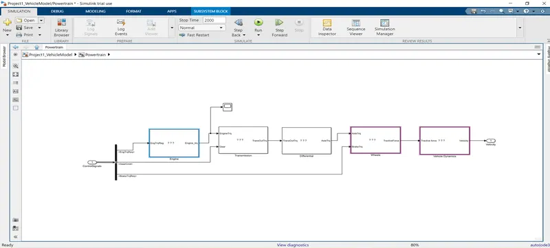
and desired brake torque. These inputs are fed to the ‘Powertrain’ block which represents the drivetrain of the vehicle. It consists of an ‘Engine’ connected to the ‘Automatic Transmission’ through a ‘Torque
Converter’. The output of the transmission is connected to the ’Differential’, which powers the ‘Wheels’, that provides the tractive force for vehicle acceleration. The longitudinal dynamics of the vehicle along with the road load is represented in the ‘Vehicle Dynamics’ block. The solver selected is ode3 with a fixed step size of 0.01 sec.
After running this Simulink model, data from the model will be loaded in the Matlab workspace.
“Project1_ProcessingFile.m” is the Matlab script used to analyze this data and to generate plots. This script needs to be executed after the Simulink model data has been loaded into the workspace. Here we
rename the variables loaded from the model (if desired), do some basic post-process calculations and generate results and plots.
Task:
The task of this project is to compute the fuel economy numbers for the given vehicle (kmpl) on the urban cycle (UDDS) and highway cycle (HWFET). Also, to analyze and understand the vehicle operating
points in terms of engine speed, torque, transmission speeds, pedal positions, gear, distance traveled, etc.
To do that, the following steps need to be followed:
1) Load the Project1 folder as the Current Folder in Matlab.
2) Run the “Project1_InitFile.m” Matlab script.
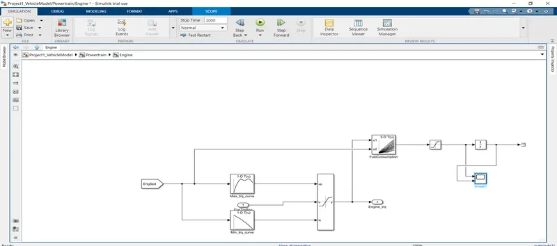
3) The provided vehicle Simulink model “Project1_VehicleModel.slx” is incomplete. The engine and vehicle dynamics block contents have been deleted. Build the Simulink blocks by referring to the course lecture and example block images provided. You can run the model and analyze the results using a ‘Scope’ for debugging.
4) Add additional ‘To Workspace’ blocks for transferring the desired Simulink vehicle data into the Matlab workspace.
5) Modify the “Project1_ProcessingFile.m” as per the desired plots and required calculations.
6) Write a project report that contains the following:
a. Tabulate the fuel economy numbers (kmpl) for UDDS and HWFET cycle. This forms the baseline numbers for comparing with the future hybrid version.
b. Plot the time trace for engine, transmission input, transmission output and wheel speed on one plot.
c. Plot engine torque, engine power, fuel rate and fuel consumption using subplots.
d. Plot accelerator and brake pedal, gear command, vehicle desired and actual speed, vehicle distance using subplots.
e. Plot the engine operating points on the engine fuel map.
f. Write down appropriate brief comments on each of these plots, describing the vehicle behavior throughout the drive cycle.
g. Generate the plots for both drive cycles