Project 1
Data cleaning on Automobile 1985 dataset and perform descriptive analytics
1. Data Importing:
# "Importing the Required libraries"
import numpy as np
import pandas as pd

# 'Importing the Dataset using Pandas'
df_auto = pd.read_csv("auto.csv", header = None)

# 'Printing the first 5 rows in the Data Frame'
df_auto.head()
Out[1]:
| 0 | 1 | 2 | 3 | 4 | 5 | 6 | 7 | 8 | 9 | ... | 16 | 17 | 18 | 19 | 20 | 21 | 22 | 23 | 24 | 25 | |
|---|---|---|---|---|---|---|---|---|---|---|---|---|---|---|---|---|---|---|---|---|---|
| 0 | 3 | ? | alfa-romero | gas | std | two | convertible | rwd | front | 88.6 | ... | 130 | mpfi | 3.47 | 2.68 | 9.0 | 111 | 5000 | 21 | 27 | 13495 |
| 1 | 3 | ? | alfa-romero | gas | std | two | convertible | rwd | front | 88.6 | ... | 130 | mpfi | 3.47 | 2.68 | 9.0 | 111 | 5000 | 21 | 27 | 16500 |
| 2 | 1 | ? | alfa-romero | gas | std | two | hatchback | rwd | front | 94.5 | ... | 152 | mpfi | 2.68 | 3.47 | 9.0 | 154 | 5000 | 19 | 26 | 16500 |
| 3 | 2 | 164 | audi | gas | std | four | sedan | fwd | front | 99.8 | ... | 109 | mpfi | 3.19 | 3.4 | 10.0 | 102 | 5500 | 24 | 30 | 13950 |
| 4 | 2 | 164 | audi | gas | std | four | sedan | 4wd | front | 99.4 | ... | 136 | mpfi | 3.19 | 3.4 | 8.0 | 115 | 5500 | 18 | 22 | 17450 |
5 rows × 26 columns
# 'Fetching the correct names using file'
headers = ['symboling','normalized-losses','make','fuel-type','aspiration','num-of-doors','body-style',\
           'drive-wheels','engine-location','wheel-base','length','width','height','curb-weight','engine-type', \
           'num-of-cylinders','engine-size','fuel-system','bore','stroke','compression-ratio','horsepower', \
           'peak-rpm','city-mpg','highway-mpg','price']
# Assigning Column names to the Data Frame
df_auto.columns = headers
df_auto.columns

# 'Printing the first 5 rows in the Data Frame'
df_auto.head()
Out[2]:
5 rows × 26 columns
| symboling | normalized-losses | make | fuel-type | aspiration | num-of-doors | body-style | drive-wheels | engine-location | wheel-base | ... | engine-size | fuel-system | bore | stroke | compression-ratio | horsepower | peak-rpm | city-mpg | highway-mpg | price | |
|---|---|---|---|---|---|---|---|---|---|---|---|---|---|---|---|---|---|---|---|---|---|
| 0 | 3 | ? | alfa-romero | gas | std | two | convertible | rwd | front | 88.6 | ... | 130 | mpfi | 3.47 | 2.68 | 9.0 | 111 | 5000 | 21 | 27 | 13495 |
| 1 | 3 | ? | alfa-romero | gas | std | two | convertible | rwd | front | 88.6 | ... | 130 | mpfi | 3.47 | 2.68 | 9.0 | 111 | 5000 | 21 | 27 | 16500 |
| 2 | 1 | ? | alfa-romero | gas | std | two | hatchback | rwd | front | 94.5 | ... | 152 | mpfi | 2.68 | 3.47 | 9.0 | 154 | 5000 | 19 | 26 | 16500 |
| 3 | 2 | 164 | audi | gas | std | four | sedan | fwd | front | 99.8 | ... | 109 | mpfi | 3.19 | 3.4 | 10.0 | 102 | 5500 | 24 | 30 | 13950 |
| 4 | 2 | 164 | audi | gas | std | four | sedan | 4wd | front | 99.4 | ... | 136 | mpfi | 3.19 | 3.4 | 8.0 | 115 | 5500 | 18 | 22 | 17450 |
# 'Saving the CSV to Local'
df_auto.to_csv('autoclean_df.csv', index = False)
The new dataset file is saved to local system.
2. Data Cleaning:
Importing the new data set to identify and fix missing values.
# 'Importing the required Libraries'
import pandas as pd
import numpy as np
import matplotlib.pylab as plt

# 'Importing the new Dataset using Pandas'
df_auto1 = pd.read_csv("autoclean_df.csv", header = None)

# 'Printing the first 5 rows in the Data Frame'
df_auto1.head()
Out[3]:
| symboling | normalized-losses | make | fuel-type | aspiration | num-of-doors | body-style | drive-wheels | engine-location | wheel-base | ... | engine-size | fuel-system | bore | stroke | compression-ratio | horsepower | peak-rpm | city-mpg | highway-mpg | price | |
|---|---|---|---|---|---|---|---|---|---|---|---|---|---|---|---|---|---|---|---|---|---|
| 0 | 3 | ? | alfa-romero | gas | std | two | convertible | rwd | front | 88.6 | ... | 130 | mpfi | 3.47 | 2.68 | 9.0 | 111 | 5000 | 21 | 27 | 13495 |
| 1 | 3 | ? | alfa-romero | gas | std | two | convertible | rwd | front | 88.6 | ... | 130 | mpfi | 3.47 | 2.68 | 9.0 | 111 | 5000 | 21 | 27 | 16500 |
| 2 | 1 | ? | alfa-romero | gas | std | two | hatchback | rwd | front | 94.5 | ... | 152 | mpfi | 2.68 | 3.47 | 9.0 | 154 | 5000 | 19 | 26 | 16500 |
| 3 | 2 | 164 | audi | gas | std | four | sedan | fwd | front | 99.8 | ... | 109 | mpfi | 3.19 | 3.4 | 10.0 | 102 | 5500 | 24 | 30 | 13950 |
| 4 | 2 | 164 | audi | gas | std | four | sedan | 4wd | front | 99.4 | ... | 136 | mpfi | 3.19 | 3.4 | 8.0 | 115 | 5500 | 18 | 22 | 17450 |
5 rows × 26 columns
# 'Identifying and Handling Missing Values'
df_auto1.replace('?', np.nan, inplace = True)
df_auto1.head()
Out[4]:
| symboling | normalized-losses | make | fuel-type | aspiration | num-of-doors | body-style | drive-wheels | engine-location | wheel-base | ... | engine-size | fuel-system | bore | stroke | compression-ratio | horsepower | peak-rpm | city-mpg | highway-mpg | price | |
|---|---|---|---|---|---|---|---|---|---|---|---|---|---|---|---|---|---|---|---|---|---|
| 0 | 3 | NaN | alfa-romero | gas | std | two | convertible | rwd | front | 88.6 | ... | 130 | mpfi | 3.47 | 2.68 | 9.0 | 111 | 5000 | 21 | 27 | 13495 |
| 1 | 3 | NaN | alfa-romero | gas | std | two | convertible | rwd | front | 88.6 | ... | 130 | mpfi | 3.47 | 2.68 | 9.0 | 111 | 5000 | 21 | 27 | 16500 |
| 2 | 1 | NaN | alfa-romero | gas | std | two | hatchback | rwd | front | 94.5 | ... | 152 | mpfi | 2.68 | 3.47 | 9.0 | 154 | 5000 | 19 | 26 | 16500 |
| 3 | 2 | 164 | audi | gas | std | four | sedan | fwd | front | 99.8 | ... | 109 | mpfi | 3.19 | 3.4 | 10.0 | 102 | 5500 | 24 | 30 | 13950 |
| 4 | 2 | 164 | audi | gas | std | four | sedan | 4wd | front | 99.4 | ... | 136 | mpfi | 3.19 | 3.4 | 8.0 | 115 | 5500 | 18 | 22 | 17450 |
5 rows × 26 columns
# 'Check for missing Data in Data Frame'
missing_data = df_auto1.isnull()
missing_data.head()
Out[5]:
| symboling | normalized-losses | make | fuel-type | aspiration | num-of-doors | body-style | drive-wheels | engine-location | wheel-base | ... | engine-size | fuel-system | bore | stroke | compression-ratio | horsepower | peak-rpm | city-mpg | highway-mpg | price | |
|---|---|---|---|---|---|---|---|---|---|---|---|---|---|---|---|---|---|---|---|---|---|
| 0 | False | True | False | False | False | False | False | False | False | False | ... | False | False | False | False | False | False | False | False | False | False |
| 1 | False | True | False | False | False | False | False | False | False | False | ... | False | False | False | False | False | False | False | False | False | False |
| 2 | False | True | False | False | False | False | False | False | False | False | ... | False | False | False | False | False | False | False | False | False | False |
| 3 | False | False | False | False | False | False | False | False | False | False | ... | False | False | False | False | False | False | False | False | False | False |
| 4 | False | False | False | False | False | False | False | False | False | False | ... | False | False | False | False | False | False | False | False | False | False |
5 rows × 26 columns
# 'Counting Missing Data in Each Column'
for col in missing_data.columns.values.tolist():
    print('Column: ', col)
    print(missing_data[col].value_counts())
    print('----------')
Out[6]:
Column:  symboling
False    205
Name: symboling, dtype: int64
----------
Column:  normalized-losses
False    164
True      41
Name: normalized-losses, dtype: int64
----------
Column:  make
False    205
Name: make, dtype: int64
----------
Column:  fuel-type
False    205
Name: fuel-type, dtype: int64
----------
Column:  aspiration
False    205
Name: aspiration, dtype: int64
----------
Column:  num-of-doors
False    203
True       2
Name: num-of-doors, dtype: int64
----------
Column:  body-style
False    205
Name: body-style, dtype: int64
----------
Column:  drive-wheels
False    205
Name: drive-wheels, dtype: int64
----------
Column:  engine-location
False    205
Name: engine-location, dtype: int64
----------
Column:  wheel-base
False    205
Name: wheel-base, dtype: int64
----------
Column:  length
False    205
Name: length, dtype: int64
----------
Column:  width
False    205
Name: width, dtype: int64
----------
Column:  height
False    205
Name: height, dtype: int64
----------
Column:  curb-weight
False    205
Name: curb-weight, dtype: int64
----------
Column:  engine-type
False    205
Name: engine-type, dtype: int64
----------
Column:  num-of-cylinders
False    205
Name: num-of-cylinders, dtype: int64
----------
Column:  engine-size
False    205
Name: engine-size, dtype: int64
----------
Column:  fuel-system
False    205
Name: fuel-system, dtype: int64
----------
Column:  bore
False    201
True       4
Name: bore, dtype: int64
----------
Column:  stroke
False    201
True       4
Name: stroke, dtype: int64
----------
Column:  compression-ratio
False    205
Name: compression-ratio, dtype: int64
----------
Column:  horsepower
False    203
True       2
Name: horsepower, dtype: int64
----------
Column:  peak-rpm
False    203
True       2
Name: peak-rpm, dtype: int64
----------
Column:  city-mpg
False    205
Name: city-mpg, dtype: int64
----------
Column:  highway-mpg
False    205
Name: highway-mpg, dtype: int64
----------
Column:  price
False    201
True       4
Name: price, dtype: int64
----------
From the output it is clear that the following missing values in each column:
1. normalized-losses (41 Records)
2. num-of-doors (2 records)
3. bore (4 records)
4. stroke (4 records)
5. horsepower (2 records)
6. peak-rpm (2 records)
7. price (4 records)
# 'Identify which method to apply to which data'
df_auto1[['normalized-losses', 'bore', 'stroke', 'horsepower', 'peak-rpm', 'num-of-doors', 'price']].head()
Out[7]:
| normalized-losses | bore | stroke | horsepower | peak-rpm | num-of-doors | price | |
|---|---|---|---|---|---|---|---|
| 0 | NaN | 3.47 | 2.68 | 111 | 5000 | two | 13495 |
| 1 | NaN | 3.47 | 2.68 | 111 | 5000 | two | 16500 |
| 2 | NaN | 2.68 | 3.47 | 154 | 5000 | two | 16500 |
| 3 | 164 | 3.19 | 3.4 | 102 | 5500 | four | 13950 |
| 4 | 164 | 3.19 | 3.4 | 115 | 5500 | four | 17450 |
After finding the missing values we need to fix the values by following method :
Replace by Mean
- normalized-losses (41 Records)
- bore (4 records)
- stroke (4 records)
- horsepower (2 records)
- peak-rpm (2 records)
Replace by Frequency
- num-of-doors (2 records)
Drop the Entire row
- price (4 records)
# 'Fixing Price Data (Drop the Entire row)'
df_auto1.dropna(subset = ['price'], axis = 0, inplace = True)
df_auto1.reset_index(drop=True, inplace=True)
df_auto1.shape
Out[8]:
(201, 26)
# 'Replace by Frequency'
    # Fixing num-of-doors variable
print(df_auto1['num-of-doors'].value_counts())

    # 'Printing what value occures the most'
print('\nTop Freq: ', df_auto1['num-of-doors'].value_counts().idxmax())

    # 'Replacing the NaN values with 'four''
df_auto1['num-of-doors'].replace(np.nan,"four", inplace = True)

    # 'Verifying if NaN removed'
df_auto1['num-of-doors'].isnull().value_counts()
Out[9]:
four 113
two 86
Name: num-of-doors, dtype: int64
Top Freq: four
False 201
Name: num-of-doors, dtype: int64
# Replace missing values by Mean
#- normalized-losses (41 Records)  --> Object type --> Convert to Float
#- bore (4 records)
#- stroke (4 records)
#- horsepower (2 records)
#- peak-rpm (2 records)

replace_by_mean  = ['normalized-losses', 'bore', 'stroke', 'horsepower', 'peak-rpm']
for i in replace_by_mean:
    mean_value = df_auto1[i].astype('float').mean()
    df_auto1[i].replace(np.nan, mean_value, inplace = True)

# Validating if the values are replaced
test_data = df_auto1[['normalized-losses', 'bore', 'stroke', 'horsepower', 'peak-rpm']].isnull()

for i in replace_by_mean:
    print(test_data[i].value_counts())

df_auto1.head()
Out[10]:
| symboling | normalized-losses | make | fuel-type | aspiration | num-of-doors | body-style | drive-wheels | engine-location | wheel-base | ... | engine-size | fuel-system | bore | stroke | compression-ratio | horsepower | peak-rpm | city-mpg | highway-mpg | price | |
|---|---|---|---|---|---|---|---|---|---|---|---|---|---|---|---|---|---|---|---|---|---|
| 0 | 3 | 122 | alfa-romero | gas | std | two | convertible | rwd | front | 88.6 | ... | 130 | mpfi | 3.47 | 2.68 | 9.0 | 111 | 5000 | 21 | 27 | 13495 |
| 1 | 3 | 122 | alfa-romero | gas | std | two | convertible | rwd | front | 88.6 | ... | 130 | mpfi | 3.47 | 2.68 | 9.0 | 111 | 5000 | 21 | 27 | 16500 |
| 2 | 1 | 122 | alfa-romero | gas | std | two | hatchback | rwd | front | 94.5 | ... | 152 | mpfi | 2.68 | 3.47 | 9.0 | 154 | 5000 | 19 | 26 | 16500 |
| 3 | 2 | 164 | audi | gas | std | four | sedan | fwd | front | 99.8 | ... | 109 | mpfi | 3.19 | 3.4 | 10.0 | 102 | 5500 | 24 | 30 | 13950 |
| 4 | 2 | 164 | audi | gas | std | four | sedan | 4wd | front | 99.4 | ... | 136 | mpfi | 3.19 | 3.4 | 8.0 | 115 | 5500 | 18 | 22 | 17450 |
5 rows × 26 columns
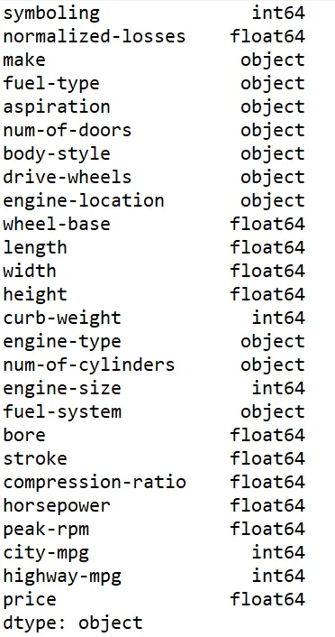
# 'Converting the above Object types to Float'
for i in replace_by_mean:
    df_auto1[[i]] = df_auto1[[i]].astype('float')

# 'Coverting the Price Valriable'
df_auto1[['price']] = df_auto1[['price']].astype('float')

# 'Verifying the Data types in Data Frame'
print(df_auto1.dtypes)
df_auto1.head(3)
Out[11]:
| symboling | normalized-losses | make | fuel-type | aspiration | num-of-doors | body-style | drive-wheels | engine-location | wheel-base | ... | engine-size | fuel-system | bore | stroke | compression-ratio | horsepower | peak-rpm | city-mpg | highway-mpg | price | |
|---|---|---|---|---|---|---|---|---|---|---|---|---|---|---|---|---|---|---|---|---|---|
| 0 | 3 | 122.0 | alfa-romero | gas | std | two | convertible | rwd | front | 88.6 | ... | 130 | mpfi | 3.47 | 2.68 | 9.0 | 111.0 | 5000.0 | 21 | 27 | 13495.0 |
| 1 | 3 | 122.0 | alfa-romero | gas | std | two | convertible | rwd | front | 88.6 | ... | 130 | mpfi | 3.47 | 2.68 | 9.0 | 111.0 | 5000.0 | 21 | 27 | 16500.0 |
| 2 | 1 | 122.0 | alfa-romero | gas | std | two | hatchback | rwd | front | 94.5 | ... | 152 | mpfi | 2.68 | 3.47 | 9.0 | 154.0 | 5000.0 | 19 | 26 | 16500.0 |
3 rows × 26 columns
# Creating Dummy Variable for Fuel Type and adding it back to the Dataset
fuel_dummy = pd.get_dummies(df_auto1['fuel-type'])
fuel_dummy.head()
Out[12]:
| diesel | gas | |
|---|---|---|
| 0 | 0 | 1 |
| 1 | 0 | 1 |
| 2 | 0 | 1 |
| 3 | 0 | 1 |
| 4 | 0 | 1 |
# 'Renaming the dummy variables to fuel-type-diesel and fuel-type-gas'
fuel_dummy.rename(columns = {'diesel': 'fuel-type-diesel', 'gas': 'fuel-type-gas'}, inplace = True)
fuel_dummy.head()
Out[13]:
| fuel-type-diesel | fuel-type-gas | |
|---|---|---|
| 0 | 0 | 1 |
| 1 | 0 | 1 |
| 2 | 0 | 1 |
| 3 | 0 | 1 |
| 4 | 0 | 1 |
# 'Saving the CSV to Local'
df_auto1.to_csv('autoclean1_df.csv', index = False)
The new dataset file is saved to local system.
3. Exploratory Data Analysis:
import pandas as pd
import numpy as np
import matplotlib.pyplot as plt
import seaborn as sns

# 'Importing the new Dataset using Pandas'
df_auto2 = pd.read_csv("autoclean1_df.csv")

df_auto2.corr()
Out[14]:
| symboling | normalized-losses | wheel-base | length | width | height | curb-weight | engine-size | bore | stroke | compression-ratio | horsepower | peak-rpm | city-mpg | highway-mpg | price | |
|---|---|---|---|---|---|---|---|---|---|---|---|---|---|---|---|---|
| symboling | 1.000000 | 0.466264 | -0.535987 | -0.365404 | -0.242423 | -0.550160 | -0.233118 | -0.110581 | -0.139896 | -0.007992 | -0.182196 | 0.075790 | 0.279719 | -0.035527 | 0.036233 | -0.082391 |
| normalized-losses | 0.466264 | 1.000000 | -0.056661 | 0.019424 | 0.086802 | -0.373737 | 0.099404 | 0.112360 | -0.029800 | 0.055127 | -0.114713 | 0.217300 | 0.239544 | -0.225016 | -0.181877 | 0.133999 |
| wheel-base | -0.535987 | -0.056661 | 1.000000 | 0.876024 | 0.814507 | 0.590742 | 0.782097 | 0.572027 | 0.493203 | 0.157964 | 0.250313 | 0.371250 | -0.360233 | -0.470606 | -0.543304 | 0.584642 |
| length | -0.365404 | 0.019424 | 0.876024 | 1.000000 | 0.857170 | 0.492063 | 0.880665 | 0.685025 | 0.608941 | 0.123913 | 0.159733 | 0.579731 | -0.286035 | -0.665192 | -0.698142 | 0.690628 |
| width | -0.242423 | 0.086802 | 0.814507 | 0.857170 | 1.000000 | 0.306002 | 0.866201 | 0.729436 | 0.544879 | 0.188814 | 0.189867 | 0.615006 | -0.245852 | -0.633531 | -0.680635 | 0.751265 |
| height | -0.550160 | -0.373737 | 0.590742 | 0.492063 | 0.306002 | 1.000000 | 0.307581 | 0.074694 | 0.180327 | -0.060822 | 0.259737 | -0.086941 | -0.309913 | -0.049800 | -0.104812 | 0.135486 |
| curb-weight | -0.233118 | 0.099404 | 0.782097 | 0.880665 | 0.866201 | 0.307581 | 1.000000 | 0.849072 | 0.644041 | 0.167412 | 0.156433 | 0.757994 | -0.279350 | -0.749543 | -0.794889 | 0.834415 |
| engine-size | -0.110581 | 0.112360 | 0.572027 | 0.685025 | 0.729436 | 0.074694 | 0.849072 | 1.000000 | 0.572516 | 0.205806 | 0.028889 | 0.822649 | -0.256753 | -0.650546 | -0.679571 | 0.872335 |
| bore | -0.139896 | -0.029800 | 0.493203 | 0.608941 | 0.544879 | 0.180327 | 0.644041 | 0.572516 | 1.000000 | -0.055390 | 0.001250 | 0.566838 | -0.267338 | -0.582121 | -0.591390 | 0.543154 |
| stroke | -0.007992 | 0.055127 | 0.157964 | 0.123913 | 0.188814 | -0.060822 | 0.167412 | 0.205806 | -0.055390 | 1.000000 | 0.187854 | 0.097815 | -0.063720 | -0.034079 | -0.034741 | 0.082267 |
| compression-ratio | -0.182196 | -0.114713 | 0.250313 | 0.159733 | 0.189867 | 0.259737 | 0.156433 | 0.028889 | 0.001250 | 0.187854 | 1.000000 | -0.214431 | -0.435721 | 0.331425 | 0.268465 | 0.071107 |
| horsepower | 0.075790 | 0.217300 | 0.371250 | 0.579731 | 0.615006 | -0.086941 | 0.757994 | 0.822649 | 0.566838 | 0.097815 | -0.214431 | 1.000000 | 0.107882 | -0.822138 | -0.804587 | 0.809681 |
| peak-rpm | 0.279719 | 0.239544 | -0.360233 | -0.286035 | -0.245852 | -0.309913 | -0.279350 | -0.256753 | -0.267338 | -0.063720 | -0.435721 | 0.107882 | 1.000000 | -0.115358 | -0.058605 | -0.101542 |
| city-mpg | -0.035527 | -0.225016 | -0.470606 | -0.665192 | -0.633531 | -0.049800 | -0.749543 | -0.650546 | -0.582121 | -0.034079 | 0.331425 | -0.822138 | -0.115358 | 1.000000 | 0.972044 | -0.686571 |
| highway-mpg | 0.036233 | -0.181877 | -0.543304 | -0.698142 | -0.680635 | -0.104812 | -0.794889 | -0.679571 | -0.591390 | -0.034741 | 0.268465 | -0.804587 | -0.058605 | 0.972044 | 1.000000 | -0.704692 |
| price | -0.082391 | 0.133999 | 0.584642 | 0.690628 | 0.751265 | 0.135486 | 0.834415 | 0.872335 | 0.543154 | 0.082267 | 0.071107 | 0.809681 | -0.101542 | -0.686571 | -0.704692 | 1.000000 |
let's find out the variable that influence the price
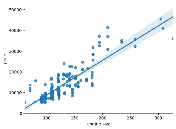
# Engine size as potential predictor variable of price
sns.regplot(x="engine-size", y="price", data=df_auto2)
plt.ylim(0,)
plt.show()
Out[15]:
(0.0, 53546.217412832855)
# 'Findng the  corelation with engine size an price'
df_auto2[["engine-size", "price"]].corr()
Out[16]:
| engine-size | price | |
|---|---|---|
| engine-size | 1.000000 | 0.872335 |
| price | 0.872335 | 1.000000 |
The Corelation between the engine size and price is about 0.87.
let see some other variables also
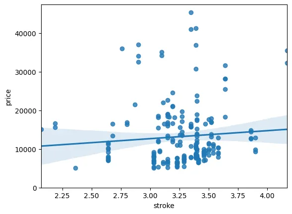
# stroke as potential predictor variable of price
sns.regplot(x="stroke", y="price", data=df_auto2)
plt.ylim(0,)
plt.show()
# 'Findng the corelation with stroke and price'
df_auto2[["stroke", "price"]].corr()
Out[17]:
| stroke | price | |
|---|---|---|
| stroke | 1.000000 | 0.082267 |
| price | 0.082267 | 1.000000 |
The Corelation between the stroke and price is about 0.082.
# drive-wheels,engine-location,body-style as potential predictor variable of price
sns.boxplot(x="drive-wheels", y="price", data=df_auto2)
plt.show()
sns.boxplot(x="engine-location", y="price", data=df_auto2)
plt.show()
sns.boxplot(x="body-style", y="price", data=df_auto2)
plt.show()
Out[18]:
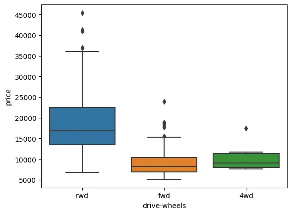
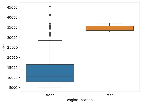
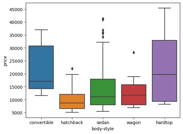
From the above results the drive-wheels might be the potential predictor for price because the distribution of price differ along the catagories.
4. Descriptive Statistical Analysis:
df_auto2.describe()
df_auto2.describe(include=['object'])
df_auto2['drive-wheels'].value_counts().to_frame()
Out[19]:
| symboling | normalized-losses | wheel-base | length | width | height | curb-weight | engine-size | bore | stroke | compression-ratio | horsepower | peak-rpm | city-mpg | highway-mpg | price | |
|---|---|---|---|---|---|---|---|---|---|---|---|---|---|---|---|---|
| count | 201.000000 | 201.00000 | 201.000000 | 201.000000 | 201.000000 | 201.000000 | 201.000000 | 201.000000 | 201.000000 | 201.000000 | 201.000000 | 201.000000 | 201.000000 | 201.000000 | 201.000000 | 201.000000 |
| mean | 0.840796 | 122.00000 | 98.797015 | 174.200995 | 65.889055 | 53.766667 | 2555.666667 | 126.875622 | 3.330711 | 3.256904 | 10.164279 | 103.396985 | 5117.587940 | 25.179104 | 30.686567 | 13207.129353 |
| std | 1.254802 | 31.99625 | 6.066366 | 12.322175 | 2.101471 | 2.447822 | 517.296727 | 41.546834 | 0.268072 | 0.316048 | 4.004965 | 37.365602 | 478.113178 | 6.423220 | 6.815150 | 7947.066342 |
| min | -2.000000 | 65.00000 | 86.600000 | 141.100000 | 60.300000 | 47.800000 | 1488.000000 | 61.000000 | 2.540000 | 2.070000 | 7.000000 | 48.000000 | 4150.000000 | 13.000000 | 16.000000 | 5118.000000 |
| 25% | 0.000000 | 101.00000 | 94.500000 | 166.800000 | 64.100000 | 52.000000 | 2169.000000 | 98.000000 | 3.150000 | 3.110000 | 8.600000 | 70.000000 | 4800.000000 | 19.000000 | 25.000000 | 7775.000000 |
| 50% | 1.000000 | 122.00000 | 97.000000 | 173.200000 | 65.500000 | 54.100000 | 2414.000000 | 120.000000 | 3.310000 | 3.290000 | 9.000000 | 95.000000 | 5117.587940 | 24.000000 | 30.000000 | 10295.000000 |
| 75% | 2.000000 | 137.00000 | 102.400000 | 183.500000 | 66.600000 | 55.500000 | 2926.000000 | 141.000000 | 3.580000 | 3.410000 | 9.400000 | 116.000000 | 5500.000000 | 30.000000 | 34.000000 | 16500.000000 |
| max | 3.000000 | 256.00000 | 120.900000 | 208.100000 | 72.000000 | 59.800000 | 4066.000000 | 326.000000 | 3.940000 | 4.170000 | 23.000000 | 262.000000 | 6600.000000 | 49.000000 | 54.000000 | 45400.000000 |
| make | fuel-type | aspiration | num-of-doors | body-style | drive-wheels | engine-location | engine-type | num-of-cylinders | fuel-system | |
|---|---|---|---|---|---|---|---|---|---|---|
| count | 201 | 201 | 201 | 201 | 201 | 201 | 201 | 201 | 201 | 201 |
| unique | 22 | 2 | 2 | 2 | 5 | 3 | 2 | 6 | 7 | 8 |
| top | toyota | gas | std | four | sedan | fwd | front | ohc | four | mpfi |
| freq | 32 | 181 | 165 | 115 | 94 | 118 | 198 | 145 | 157 | 92 |
| drive-wheels | |
|---|---|
| fwd | 118 |
| rwd | 75 |
| 4wd | 8 |
# 'grouping results'
df_gptest = df_auto2[['drive-wheels','body-style','price']]
grouped_test1 = df_gptest.groupby(['drive-wheels','body-style'],as_index=False).mean()
grouped_test1# grouping results
df_gptest = df_auto2[['drive-wheels','body-style','price']]
grouped_test1 = df_gptest.groupby(['drive-wheels','body-style'],as_index=False).mean()
grouped_test1

df_auto2.corr()
Out[20]:
| drive-wheels | body-style | price | |
|---|---|---|---|
| 0 | 4wd | hatchback | 7603.000000 |
| 1 | 4wd | sedan | 12647.333333 |
| 2 | 4wd | wagon | 9095.750000 |
| 3 | fwd | convertible | 11595.000000 |
| 4 | fwd | hardtop | 8249.000000 |
| 5 | fwd | hatchback | 8396.387755 |
| 6 | fwd | sedan | 9811.800000 |
| 7 | fwd | wagon | 9997.333333 |
| 8 | rwd | convertible | 23949.600000 |
| 9 | rwd | hardtop | 24202.714286 |
| 10 | rwd | hatchback | 14337.777778 |
| 11 | rwd | sedan | 21711.833333 |
| 12 | rwd | wagon | 16994.222222 |
| symboling | normalized-losses | wheel-base | length | width | height | curb-weight | engine-size | bore | stroke | compression-ratio | horsepower | peak-rpm | city-mpg | highway-mpg | price | |
|---|---|---|---|---|---|---|---|---|---|---|---|---|---|---|---|---|
| symboling | 1.000000 | 0.466264 | -0.535987 | -0.365404 | -0.242423 | -0.550160 | -0.233118 | -0.110581 | -0.139896 | -0.007992 | -0.182196 | 0.075790 | 0.279719 | -0.035527 | 0.036233 | -0.082391 |
| normalized-losses | 0.466264 | 1.000000 | -0.056661 | 0.019424 | 0.086802 | -0.373737 | 0.099404 | 0.112360 | -0.029800 | 0.055127 | -0.114713 | 0.217300 | 0.239544 | -0.225016 | -0.181877 | 0.133999 |
| wheel-base | -0.535987 | -0.056661 | 1.000000 | 0.876024 | 0.814507 | 0.590742 | 0.782097 | 0.572027 | 0.493203 | 0.157964 | 0.250313 | 0.371250 | -0.360233 | -0.470606 | -0.543304 | 0.584642 |
| length | -0.365404 | 0.019424 | 0.876024 | 1.000000 | 0.857170 | 0.492063 | 0.880665 | 0.685025 | 0.608941 | 0.123913 | 0.159733 | 0.579731 | -0.286035 | -0.665192 | -0.698142 | 0.690628 |
| width | -0.242423 | 0.086802 | 0.814507 | 0.857170 | 1.000000 | 0.306002 | 0.866201 | 0.729436 | 0.544879 | 0.188814 | 0.189867 | 0.615006 | -0.245852 | -0.633531 | -0.680635 | 0.751265 |
| height | -0.550160 | -0.373737 | 0.590742 | 0.492063 | 0.306002 | 1.000000 | 0.307581 | 0.074694 | 0.180327 | -0.060822 | 0.259737 | -0.086941 | -0.309913 | -0.049800 | -0.104812 | 0.135486 |
| curb-weight | -0.233118 | 0.099404 | 0.782097 | 0.880665 | 0.866201 | 0.307581 | 1.000000 | 0.849072 | 0.644041 | 0.167412 | 0.156433 | 0.757994 | -0.279350 | -0.749543 | -0.794889 | 0.834415 |
| engine-size | -0.110581 | 0.112360 | 0.572027 | 0.685025 | 0.729436 | 0.074694 | 0.849072 | 1.000000 | 0.572516 | 0.205806 | 0.028889 | 0.822649 | -0.256753 | -0.650546 | -0.679571 | 0.872335 |
| bore | -0.139896 | -0.029800 | 0.493203 | 0.608941 | 0.544879 | 0.180327 | 0.644041 | 0.572516 | 1.000000 | -0.055390 | 0.001250 | 0.566838 | -0.267338 | -0.582121 | -0.591390 | 0.543154 |
| stroke | -0.007992 | 0.055127 | 0.157964 | 0.123913 | 0.188814 | -0.060822 | 0.167412 | 0.205806 | -0.055390 | 1.000000 | 0.187854 | 0.097815 | -0.063720 | -0.034079 | -0.034741 | 0.082267 |
| compression-ratio | -0.182196 | -0.114713 | 0.250313 | 0.159733 | 0.189867 | 0.259737 | 0.156433 | 0.028889 | 0.001250 | 0.187854 | 1.000000 | -0.214431 | -0.435721 | 0.331425 | 0.268465 | 0.071107 |
| horsepower | 0.075790 | 0.217300 | 0.371250 | 0.579731 | 0.615006 | -0.086941 | 0.757994 | 0.822649 | 0.566838 | 0.097815 | -0.214431 | 1.000000 | 0.107882 | -0.822138 | -0.804587 | 0.809681 |
| peak-rpm | 0.279719 | 0.239544 | -0.360233 | -0.286035 | -0.245852 | -0.309913 | -0.279350 | -0.256753 | -0.267338 | -0.063720 | -0.435721 | 0.107882 | 1.000000 | -0.115358 | -0.058605 | -0.101542 |
| city-mpg | -0.035527 | -0.225016 | -0.470606 | -0.665192 | -0.633531 | -0.049800 | -0.749543 | -0.650546 | -0.582121 | -0.034079 | 0.331425 | -0.822138 | -0.115358 | 1.000000 | 0.972044 | -0.686571 |
| highway-mpg | 0.036233 | -0.181877 | -0.543304 | -0.698142 | -0.680635 | -0.104812 | -0.794889 | -0.679571 | -0.591390 | -0.034741 | 0.268465 | -0.804587 | -0.058605 | 0.972044 | 1.000000 | -0.704692 |
| price | -0.082391 | 0.133999 | 0.584642 | 0.690628 | 0.751265 | 0.135486 | 0.834415 | 0.872335 | 0.543154 | 0.082267 | 0.071107 | 0.809681 | -0.101542 | -0.686571 | -0.704692 | 1.000000 |
df_gptestOut[21]:
| drive-wheels | body-style | price | |
|---|---|---|---|
| 0 | rwd | convertible | 13495.0 |
| 1 | rwd | convertible | 16500.0 |
| 2 | rwd | hatchback | 16500.0 |
| 3 | fwd | sedan | 13950.0 |
| 4 | 4wd | sedan | 17450.0 |
| ... | ... | ... | ... |
| 196 | rwd | sedan | 16845.0 |
| 197 | rwd | sedan | 19045.0 |
| 198 | rwd | sedan | 21485.0 |
| 199 | rwd | sedan | 22470.0 |
| 200 | rwd | sedan | 22625.0 |
201 rows × 3 columns
5. Conclusion:
From the we have found out the which variable is used to predict the output.
The Variables are listed down as follows:
Continuous numerical variables:
1. Length
2. Width
3. Curb-weight
4. Engine-size
5. Horsepower
6. City-mpg
7. Highway-mpg
8. Wheel-base
9. Bore
Categorical variables:
1. Drive-wheels