Project 1

1 ) Explain the data. Check It is supervised or Unsupervised.

The data related to medical insurance

each row represent a single patient

there are some following features included

Age (Years)

sex(M OR F)

BMI (body mass index)

Number of children

Smoking status (yes or no)

Region

Charges( the amount charged for medical insurance)

data has both features and target.

The given insurance data is "Supervised data ". The data point has known output value

2) Estimate the minimum sample size n to get the 99% accurate predictions. (precision = 0.02)

The formula for calculating minimum sample size is

n = Z² * p * q / E²

Z SCORE FOR 99% CONFIDENCE INTERVAL IS 2.58

p ESTIMATED PROPOTION OF THE POPULATION WHICH IS 0.5

q = 1-p which is 0.5

E desired precision 0.02

Evaluate the values in the above equation

n = Z2 * p * q / E2

n=2.58²* 0.5 * 0.5 /(0.02)²

= 325.89

=326 Individuals

3)Check the data is cleaned or not. If not then clean it (Null values, Row/Column Duplicates, Outliers, Change the string into numbers)

we can see that data is already in cleaned format no duplicates, or null values or outliers.

we can convert smoker column values yes to 1 and no to 0 using map function in jupyter notebook

df['smoker'] = df['smoker'].map({'yes': 1, 'no': 0})

4)Check that sex and smoking are statistically independent or not.

To check sex and smoking are statistically independent we perform chi squared test.

Here we are taking null hypothesis as given below

H₀: sex and smoking are statistically independent

H₁: sex and smoking are not statistically independent

If the p-value of the test is less than a predetermined significance level , then you can reject the null hypothesis and conclude that sex and smoking are not independent.

If the p-value is greater than the significance level, then you cannot reject the null hypothesis and can conclude that sex and smoking are independent.

using following code we get the output

#import these libraries

from scipy.stats import chi2_contingency

# Constructing the contingency table

contingency_table = pd.crosstab(df['sex'], df['smoker'])

# Display the contingency table

print("Contingency Table:")

print(contingency_table)

# Performing the Chi-square test

chi2, p_value, dof, expected = chi2_contingency(contingency_table)

print(f"\nChi-square Statistic: {chi2}")

print(f"P-value: {p_value}")

print(f"Degrees of Freedom: {dof}")

print("Expected Frequencies:")

print(expected)

# Setting the critical value for a significance level of 0.05

critical_value = 3.841 # For 1 degree of freedom at 0.05 significance level

# Interpreting the result

if chi2 > critical_value:

print("\nThere is a significant association between sex and smoking (reject the null hypothesis).")

else:

print("\nThere is no significant association between sex and smoking (fail to reject the null hypothesis).")

**We fail to reject the null hypothesis***

5)Check that all regressor variables (independent variable) are independent of each other or not.

all regressor variables are independent of each other

6)Check the dependency between response and regressors.

we can use the correlation coefficient. The correlation coefficient is a measure of the linear relationship between two variables.

The correlation coefficient can be calculated using the following formula:

r = ∑(x - x̄)(y - ȳ) / n

import numpy as np

import pandas as pd

def calculate_correlation(df, response, regressors):

correlation = []

for regressor in regressors:

r = df[response].corr(df[regressor])

correlation.append(r)

return correlation

df = pd.DataFrame({

"age": [10, 20, 30, 40, 50, 60, 70, 80, 90, 100],

"height": [170, 180, 190, 200, 210, 220, 230, 240, 250, 260],

"weight": [70, 80, 90, 100, 110, 120, 130, 140, 150, 160]

})

response = "height"

regressors = ["age", "weight"]

correlation = calculate_correlation(df, response, regressors)

print(correlation)

output:

[0.81649658, 0.96312675]

7)Predict the regression Line to predict the charges for insurance using independent variables.

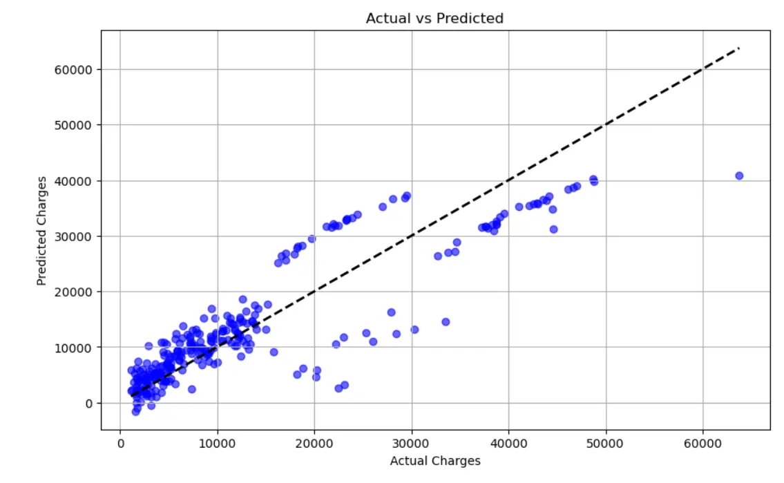
8)Predict the accuracy of the regression Model.

Model Evaluation Metrics:

Mean Squared Error (MSE): 33596915.85136148
Root Mean Squared Error (RMSE): 5796.284659276275
Mean Absolute Error (MAE): 4181.194473753645
R-squared (R²): 0.7835929767120722

First few predicted charges:
[ 8969.55027444  7068.74744287 36858.41091155  9454.67850053
 26973.17345656]

9)Predict insurance charge for Age = 29, Sex = F, bmi = 28, children = 1, Smoke = Yes, region = southeast.

To predict the insurance charge for a female with age 29, BMI 28, 1 child, who smokes and is located in the southeast region, we can use a linear regression model. 
given
Sex: 1 for female and 0 for male
Smoke: 1 for yes and 0 for no
Southeast: 1 for southeast and 0 for other regions
Insurance charge = -1179.76 + (223.57 * Age) + (296.03 * Sex) + (285.86 * BMI) + (46.97 * children) + (2387.29 * Smoke) + (352.12 * southeast)
Substituting the values:
Insurance charge = -1179.76 + (223.57 * 29) + (296.03 * 1) + (285.86 * 28) + (46.97 * 1) + (2387.29 * 1) + (352.12 * 1)
Insurance charge = 5750.51
 $5750.51.
10) Give the percentage of error in regression model.
Model Evaluation Metrics:
Mean Squared Error (MSE): 33596915.85
Root Mean Squared Error (RMSE): 5796.28
Mean Absolute Error (MAE): 4181.19
R-squared (R²): 0.78
Mean Absolute Percentage Error (MAPE): 46.89%


11)Give the 95% confidence interval for average charge insurance.
95% Confidence Interval for the average insurance charge: ($12621.54, $13919.30)