% Initialization file for loading the variables for the Conventional vehicle simulation model
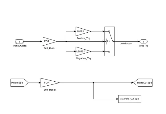
DiffEff = 0.99; % Differential efficiency (assumed independent of operating conditions)
TransEff = 0.90; % Transmission efficiency (assumed independent of operating conditions)
TC_SR = [0, .5, .6, .7, .8, .87, .92, .94, .96, .97, 1]; % Torque Converter Speed Ratio (Matlab default) -> TurbSpd/PumpSpd
TC_TR = [2.232, 1.5462, 1.4058, 1.2746, 1.1528, 1.0732, 1.0192, 1, 1, 1, 1]; % Torque Converter Torque Ratio (Matlab default) -> TurbTrq/PumpTrq
TC_Cf = 1e-4 * [.72558, .66322, .63463, .59042, .51331, .4144, .29287, .22444, .12186, .04386, 0]; % Torque Converter Capacity Factor (Matlab default) -> PumpTrq/PumpSpd^2 [Nm/rpm^2]
this Block we want ot edit clearly.
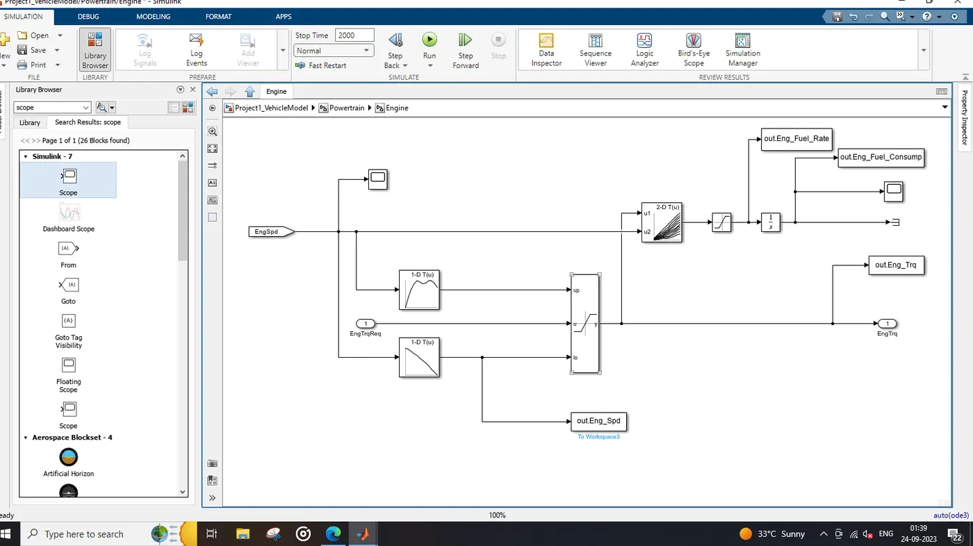
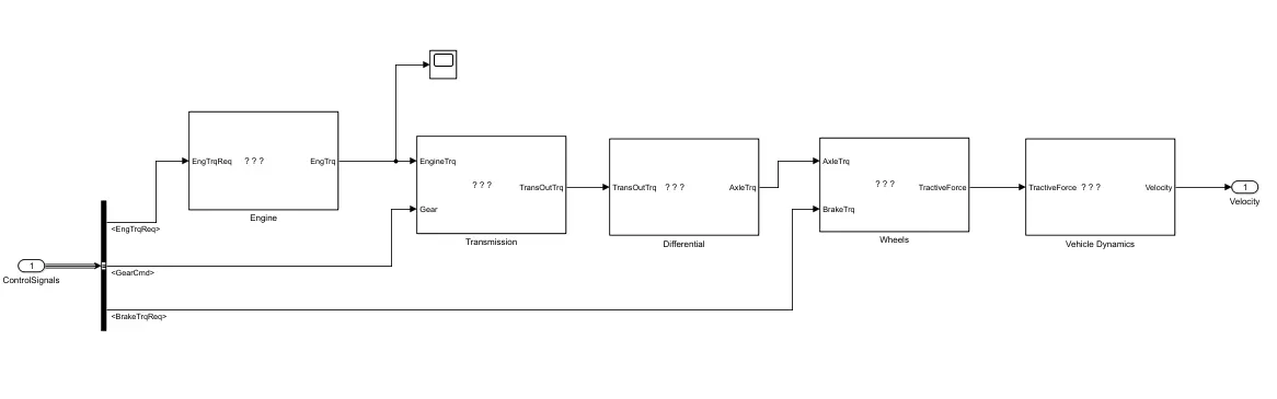
Engine and vehicle dynamic blocks are added above.
Understand each ans every block design to complete project.
%% Skill-Lync -> Hybrid Drives Development
% Project 1 - Conventional Vehicle Model
% By - Dharmesh Ravindra Bonde
�scription:
% The following file is to used with the Initialization file and Simulink
% results for post-processing of the data.
% The file is incomplete, has some examples of how the data is imported
% into a readable format, data analysis and plotting examples.
�sed on the project task, use commands in a similar format as given
�low, to analyse the data and generate required plots.
% You can change variable names if desired
%% Post-Processing File
% File for post-processing the Conventional vehicle simulation model data
%% Renaming variables
Time = out.tout;
Acc_Pdl = out.Acc_Pdl; �celerator pedal [%]
Brk_Pdl = out.Brk_Pdl; % Brake pedal [%]
Gear_Cmd = out.Gear_Cmd; % Transmission gear
Trans_In_Spd = out.Trans_In_Spd*30/pi; % Transmission input speed [rpm]
Trans_Out_Spd = out.Trans_Out_Spd*30/pi;% Transmission output speed [rpm]
Eng_Trq = out.Eng_Trq; % Engine brake torque [Nm]
Eng_Spd = out.Eng_Spd*30/pi; % Engine speed [rpm]
Eng_Fuel_consump = out.Eng_Fuel_Consump; % Engine fuel consumption [g]
Veh_Dist = out.Veh_Dist/1000; % Distance traveled by vehicle [km]
Veh_Spd = out.Veh_Spd*18/5; % Vehicle speed [kmph]
Wheel_Speed = out.wh_speed; % Wheel speed [kmph]
Eng_Fuel_Rate = out.Eng_Fuel_Rate % Engine fuel rate [%]
%�ta Analysis
Eng_Pwr = (Eng_Spd*pi/30) .* (Eng_Trq/1000); % Engine brake power [kW]
rho_petrol = 0.7197; �nsity of petrol [kg/L]
kmpl = Veh_Dist(end)/(Eng_Fuel_consump(end)/1000/rho_petrol); % Fuel economy [kmpl]
%% Plotting vehicle characteristics time trace transmission IN/OUT and Wheel Speed
figure(1)
hold on
grid on
plot(Time, Trans_In_Spd, 'linewidth', 1, 'Color', 'black');
plot(Time, Trans_Out_Spd, 'linewidth', 1, 'Color', 'red');
%plot(Time, Wheel_Speed, 'linewidth',1, 'color', 'blue')
ylabel('Speed [rpm]')
xlabel('Timem [s]')
xlim([0, Time(end)]);
ylim([0, 6000]);
legend('Trans Input','Trans Output','Wheel Speed');
%% Plotting vehicle characteristics time trace to Engine speed, Engine Torque, Engine Power,
% And Engine fuel rate, Engine fuel consumption
�ta conversion from Double Timeseries
%Eng_Spd = Eng_Spd.Data(:,1); % engine speed
%Eng_trq = Eng_Trq.Data(:,1); % engine torque
%Eng_pwr = Eng_Pwr.Data(:,1); % engine power
Eng_Fuel_Rate = out.Eng_Fuel_Rate % engine fuel rate
%Eng_fuel_consumption = Eng_Fuel_Consump.Data(:,1); % engine fuel consumption
%Veh_dist = Veh_Dist.Data(:,1); % vehicle distance
%Veh_spd = Veh_Spd.Data(:,1); % vehicle speed
% Plotting Engine speed, Engine Torque, Engine Power,Engine fuel rate,Engine fuel consumption wrt Time
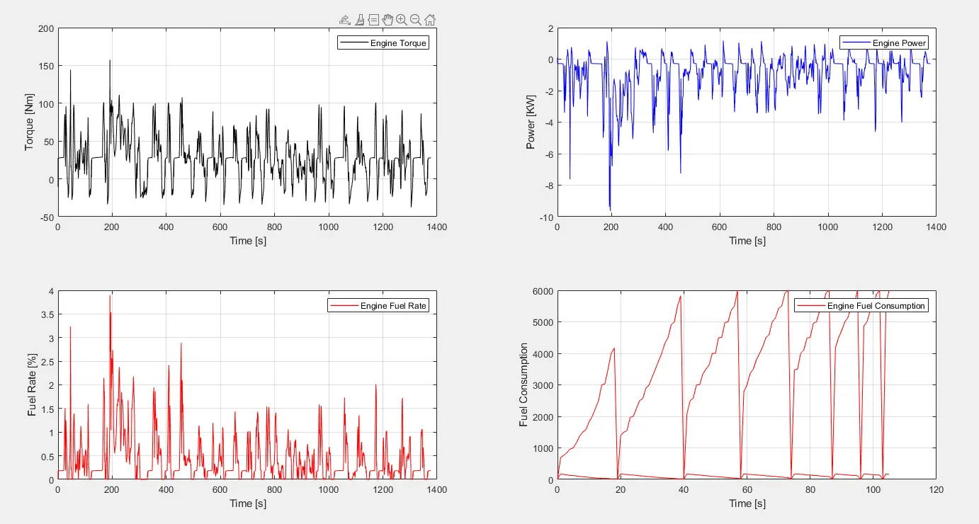
figure(2)
subplot(2,2,1)
plot(Time,Eng_Trq,'linewidth',1,'color','black')
xlabel('Time [s]')
ylabel('Torque [Nm]')
legend('Engine Torque')
grid on
subplot(2,2,2)
plot(Time,Eng_Pwr,'linewidth',1,'color','blue')
xlabel('Time [s]')
ylabel('Power [KW]')
legend('Engine Power')
grid on
subplot(2,2,3)
plot(Time,Eng_Fuel_Rate,'linewidth',1,'color','red')
xlabel('Time [s]')
ylabel('Fuel Rate [%]')
legend('Engine Fuel Rate')
grid on
subplot(2,2,4)
Time = linspace(0,105,length(c));
plot(Time,c,'linewidth',1,'color','red')
xlabel('Time [s]')
ylabel('Fuel Consumption')
legend('Engine Fuel Consumption')
grid on
% Plotting fuel economy Vs Engine Fuel consumption
figure(3)
plot(Eng_Fuel_consump,Eng_Fuel_Rate,'color','r')
xlabel('Fuel consumption')
ylabel('Fuel Rate [%]')
title('Fuel economy Vs Fuel Consumption')
grid on
%% Potting Accelerator pedal, Brake pedal and gear command with respect to time
figure(4)
subplot(2,1,1)
hold on
Time = linspace(0,137734,length(Acc_Pdl));
plot(Time, Acc_Pdl, 'linewidth', 1, 'Color', 'black');
plot(Time, Brk_Pdl, 'linewidth', 1, 'Color', 'red');
ylabel('Pedal [%]')
xlabel('Time [s]');
xlim([0, Time(end)]);
grid on
legend('Accel','Brake');
title('Acceleration & Brake Pedal wrt Time')
subplot(2,1,2)
plot(Time, Gear_Cmd, 'linewidth', 1, 'Color', 'black');
xlim([0, Time(end)]);
xlabel('Time [s]');
ylabel('Gear');
grid on
title('Gear command wrt Time')
% Plotting gear command vehicle desired with actual speed
figure(5)
subplot(2,1,1)
plot(Veh_Spd, Gear_Cmd, 'linewidth', 1, 'Color', 'black');
xlabel('Speed [rpm]');
ylabel('Gear');
grid on
title('Gear command wrt vehicle speed')
subplot(2,1,2)
p=plot(Veh_Dist, Gear_Cmd,'linewidth', 1, 'Color', 'red');
xlabel('Distance [kmpl]');
ylabel('Gear');
grid on
title('Gear command wrt Distance')
%% Plotting engine operating points on engine fuel map
figure('Name','Engine Operating Points');
hold on
grid on
title('Engine Operating Points','fontsize',12);
p1=plot(Eng_map_spd*30/pi,Eng_max_trq,'linewidth',2,'color','r');
p2=line([Eng_map_spd(end)*30/pi Eng_map_spd(end)*30/pi],[0 Eng_max_trq(end)]);
set(p2,'linewidth',1,'linestyle','--','color','k');
p3=line([Eng_map_spd(1)*30/pi Eng_map_spd(1)*30/pi],[0 Eng_max_trq(1)]);
set(p3,'linewidth',1,'linestyle','--','color','k');
[c,h] = contour(Eng_map_spd'*30/pi,Eng_map_trq,Eng_fuel_map');
clabel(c,h);
xlabel('Engine Speed [rpm]');
ylabel('Engine Torque [Nm]');
title('Engine Fuel Consumption Map [g/s]');
legend([p1 p3],{'Max Curve','Operating Points'});
axis([Eng_map_spd(1)*30/pi Eng_map_spd(end)*30/pi 0 Eng_map_trq(end)]);
output of the programe is
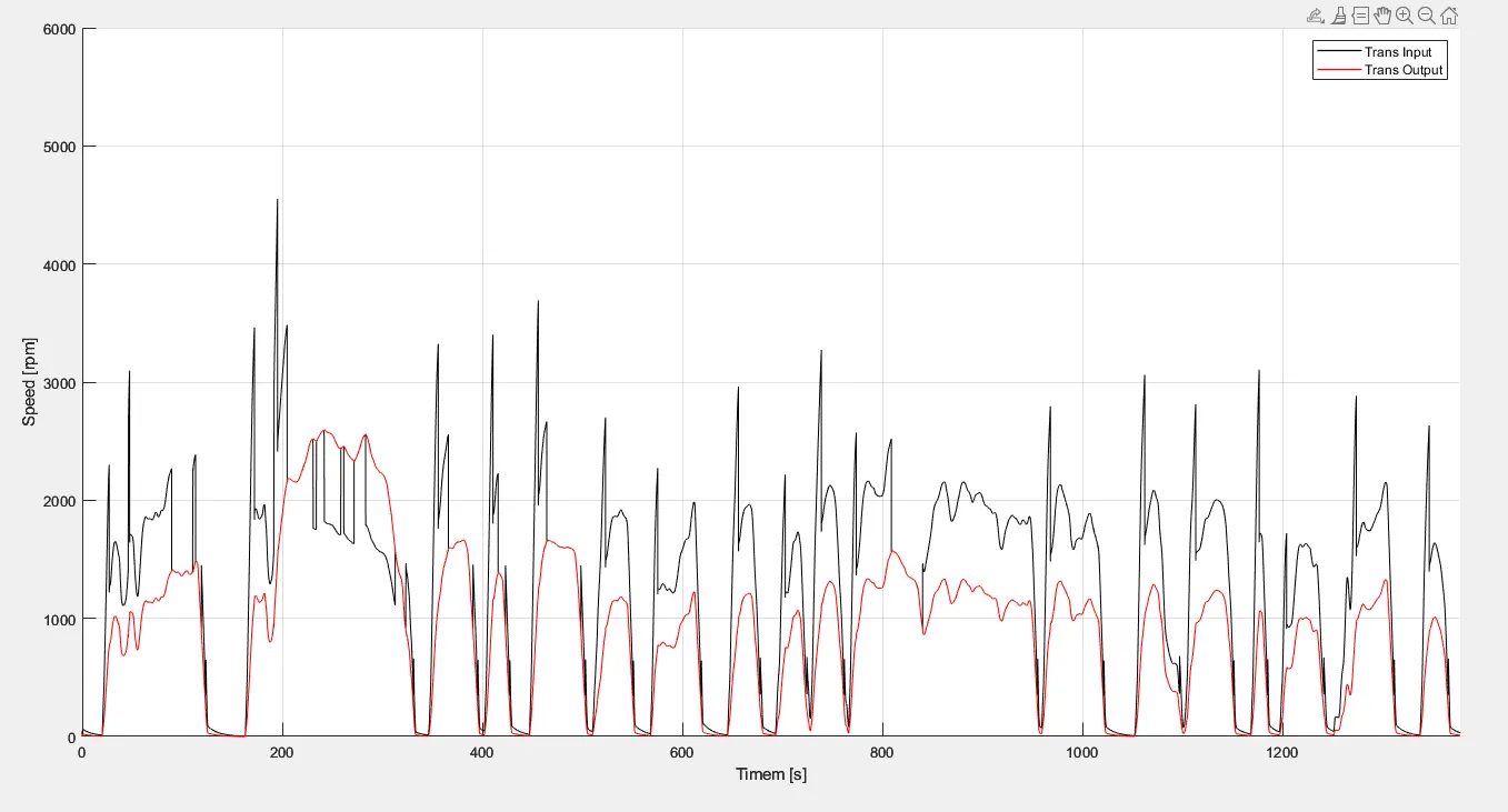
out put 1
In this graph we see the transmission input and transmission out will fluctuates up and down as increasing speed and time.
second output
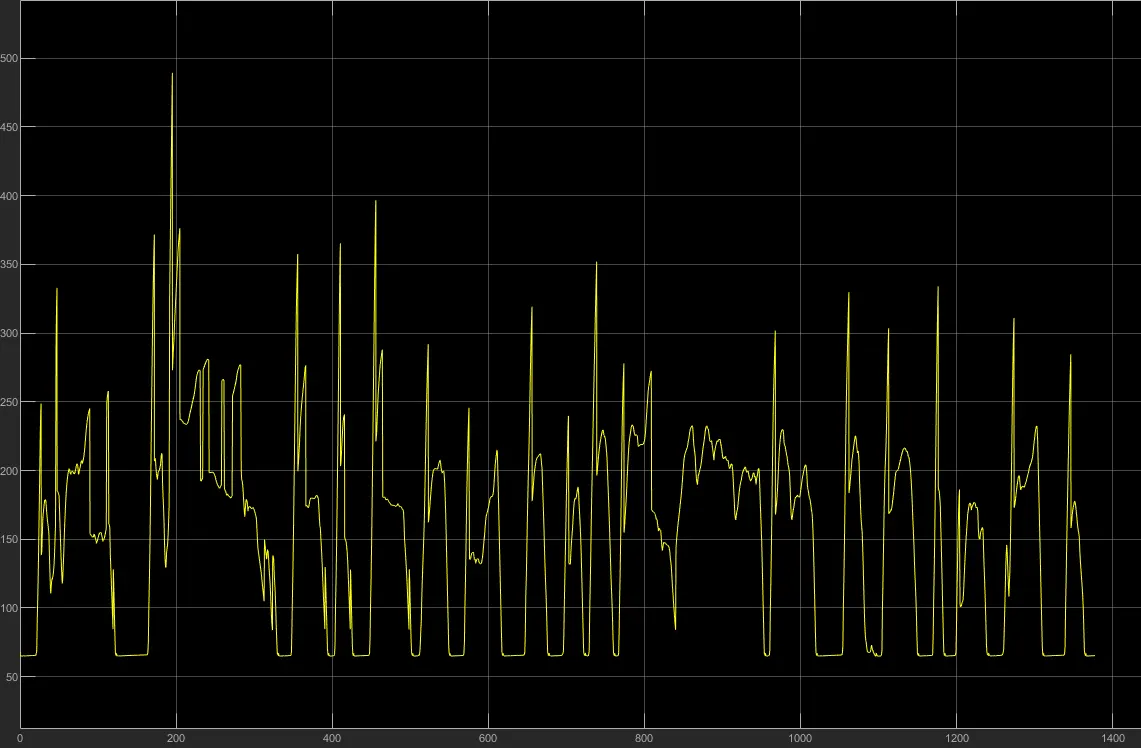
In this engine torque, Engine power, engine fuel rate and engine fuel consumption is increase increasing wrt time.
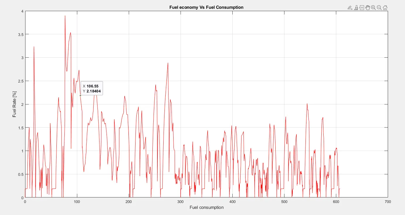
output 3
Fuel consumption vs fuel rate
 4] Potting Accelerator pedal, Brake pedal and gear command with respect to time:-
In this the as comparing brake of vehicle the accelaration of vehicle is more so the brake torque is min required. and the gear shifting is also required wrt time.
Hence the end of the programme we can abel to find the complete model of hybrid EV and it dynamic
and it future.
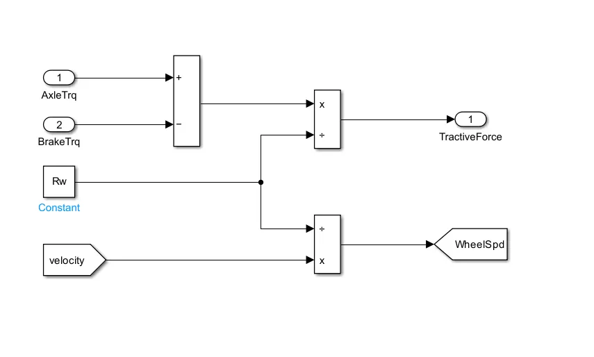
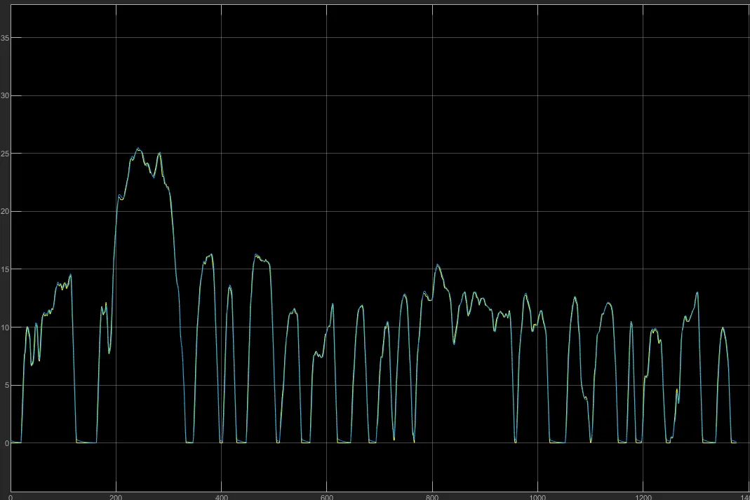
 vehicle dynamic Block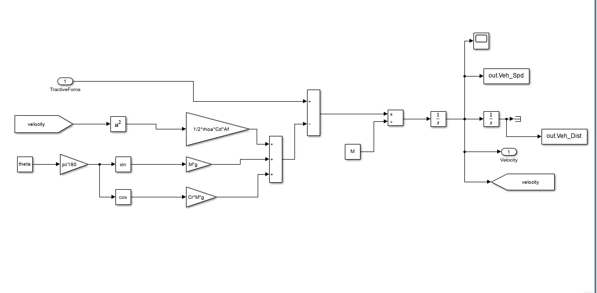
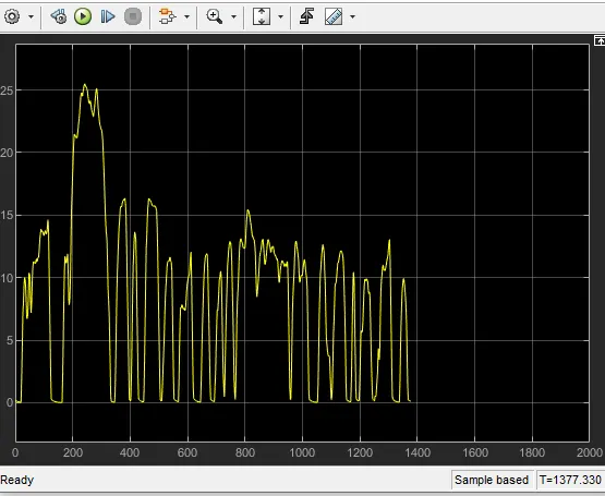
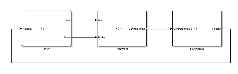
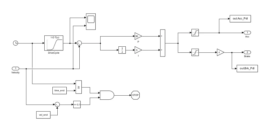
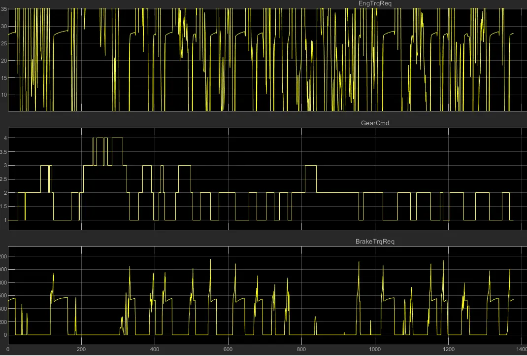
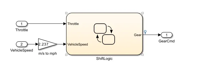
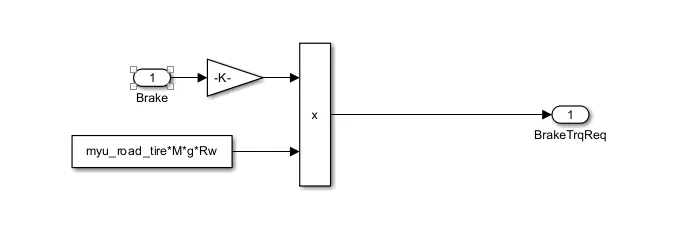
 controller block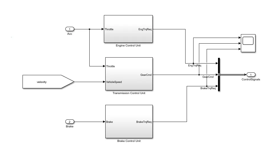
 Engine control unit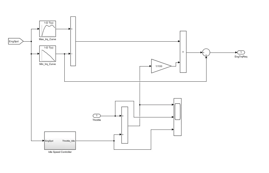
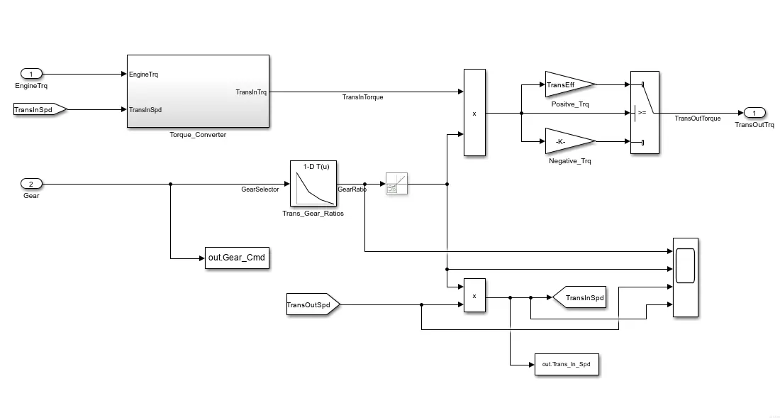
 transmission: