Project 1
PROJECT 1
The script (Project1_InitFile.m) for the project
Here the UDDS drive cycle is selected for the simulation
%% Vehicle Parameters
M = 1500; % Vehicle weight [kg]
Cr = 0.015; % Rolling resistance coefficient
Rw = 0.35; % Rolling radius [m]
Cd = 0.33; % Drag coefficient
Af = 2; % Frontal area [m2]
rhoa = 1.225; % Air density [kg/m3]
Vwind = 0; % Wind velocity [kmph]
g = 9.81; % Gravitational acceleration [m/s2]
theta = 0; % Slope [deg]
myu_road_tire = 1; % Coefficient of friction between tire-road interface
%% Powertrain Parameters
FDR = 3.73; % Final Drive Ratio / Diff Ratio
DiffEff = 0.99; % Differential efficiency (assumed independent of operating conditions)
NumGear = 4; % Number of gears in transmission
TransGear = 1:NumGear; % Transmission Gears
TransRatio = [3.06, 1.62, 1, 0.7]; % Corresponding Transmission ratios
TransEff = 0.90; % Transmission efficiency (assumed independent of operating conditions)
TC_SR = [0, .5, .6, .7, .8, .87, .92, .94, .96, .97, 1]; % Torque Converter Speed Ratio (Matlab default) -> TurbSpd/PumpSpd
TC_TR = [2.232, 1.5462, 1.4058, 1.2746, 1.1528, 1.0732, 1.0192, 1, 1, 1, 1]; % Torque Converter Torque Ratio (Matlab default) -> TurbTrq/PumpTrq
TC_Cf = 1e-4 * [.72558, .66322, .63463, .59042, .51331, .4144, .29287, .22444, .12186, .04386, 0]; % Torque Converter Capacity Factor (Matlab default) -> PumpTrq/PumpSpd^2 [Nm/rpm^2]
load Vehicle_Data/Engine_data_1_9L_Saturn_95kW
load Vehicle_Data/Trans_Shift_map
%% Driver Parameters
Kp = 10; % P gain for driver PI model
Ki = 1; % I gain for driver PI model
Drive_Cycle_Select = 1; % Drive cycle selection
% Drive cycle values in m/s
if Drive_Cycle_Select == 1
load DriveCycles/UDDS;
elseif Drive_Cycle_Select == 2
load DriveCycles/HWFET;
elseif Drive_Cycle_Select == 3
load DriveCycles/FTP;
elseif Drive_Cycle_Select == 4
load DriveCycles/US06;
elseif Drive_Cycle_Select == 5
load DriveCycles/NEDC;
elseif Drive_Cycle_Select == 6
load DriveCycles/WLTP;
end
time_end = cyc_time(end);
vel_end = cyc_vel(end);
The script (Project1_ProcessingFile.m) for the project
Time = out.tout;
Acc_Pdl = out.Acc_Pdl; Accelerator pedal [%]
Brk_Pdl = out.Brk_Pdl; % Brake pedal [%]
Gear_Cmd = out.Gear_Cmd; % Transmission gear
Trans_In_Spd = out.Trans_In_Spd*30/pi; % Transmission input speed [rpm]
Trans_Out_Spd = out.Trans_Out_Spd*30/pi;% Transmission output speed [rpm]
Eng_Fuel_ratio = out.Eng_Fuel_Ratio;% Engine fuel ratio
Eng_Trq = out.Eng_Trq; % Engine brake torque [Nm]
Eng_Spd = out.Eng_Spd*30/pi; % Engine speed [rpm]
Eng_Fuel_Consump = out.Eng_Fuel_Consumption; % Engine fuel consumption [g]
Veh_Dist = out.Veh_Dist/1000; % Distance traveled by vehicle [km]
Veh_Spd = out.Veh_Spd*18/5; % Vehicle speed [kmph]
wheel_speed = out.wheel_speed*30/pi; % wheel_speed [Rpm]
cyc_vel_km = cyc_vel*18/5; %cycle(desired) velocity in [Kmph]
�ta Analysis
Eng_Pwr = Eng_Spd.*pi./30.*Eng_Trq/1000; % Engine brake power [kW]
rho_petrol = 0.7197; Density of petrol [kg/L]
kmpl = Veh_Dist(end)/(Eng_Fuel_Consump(end)/1000/rho_petrol); % Fuel economy [kmpl]
%% (B) Plotting the time trace for engine, transmission input, transmission output and wheel speed on one plot.
figure(1)
hold on
grid minor
plot(Time, Trans_In_Spd, 'linewidth', 1, 'Color', 'black');
plot(Time, Trans_Out_Spd, 'linewidth', 1, 'Color', 'red');
plot(Time, wheel_speed,'linewidth',1,'Color','cyan');
xlabel('time trace')
ylabel('Speed [rpm]')
xlim([0, Time(end)]);
ylim([0, 6000]);
legend('Trans Input', 'Trans Output','wheel speed');
%% Plotting engine torque, engine power, fuel rate and fuel consumption using subplots.
figure(2)
subplot(2,2,1)
hold on
grid on
plot(Time,Eng_Trq, 'linewidth', 1, 'Color', 'blue');
title('Time vs Engine torque');
xlabel('Time [s]');
ylabel('Engine torque(Nm)')
xlim([0, Time(end)]);
legend('Engine torque');
subplot(2,2,2)
hold on
grid on
plot(Time,Eng_Pwr,'linewidth', 1, 'Color', 'red');
title('Time vs Engine Power');
xlabel('Time [s]');
ylabel('Eng Powerwr(KW)');
xlim([0, Time(end)]);
legend('Engine Power');
subplot(2,2,3)
hold on
grid on
plot(Time,Eng_Fuel_ratio,'linewidth', 1, 'Color', 'cyan');
title('Time vs Engine fuel ratio');
xlabel('Time [s]');
ylabel('Eng fuel ratio');
xlim([0, Time(end)]);
legend('Eng fuel ratio');
subplot(2,2,4)
hold on
grid on
plot(Time,Eng_Fuel_Consump,'linewidth', 1, 'Color', 'magenta');
title('Time vs Engine Fuel Consumption');
xlabel('Time [s]');
ylabel('Eng Fuel Consumption(g)');
xlim([0, Time(end)]);
legend('Engine Fuel Consumption');
%% Plotting accelerator and brake pedal, gear command, vehicle desired and actual speed, vehicle distance using subplots
figure(3);
subplot(4,1,1);
hold on
grid on
plot(Time,Acc_Pdl,'color','black');
plot(Time,Brk_Pdl,'color','red');
title('time vs acc and brake pedal');
xlabel('time(s)');
ylabel('pedal(%)');
legend('Accel','brake');
subplot(4,1,2);
hold on
grid on
plot(Time, Gear_Cmd,'Color', 'cyan');
xlim([0, Time(end)]);
title('time vs Gear');
xlabel('Time [s]');
ylabel('Gear');
legend('Gear command');
subplot(4,1,3);
hold on
grid on
plot(cyc_time,cyc_vel_km,'Color', 'black');
plot(Time,Veh_Spd,'Color', 'red');
title('Desired and Actual speed');
xlabel('Time');
ylabel('Speed[Kmph]');
legend('Desired speed','Actual speed');
subplot(4,1,4);
hold on
grid on
plot(Time,Veh_Dist,'Color', 'green');
title('Time vs Vehicle Distance');
xlabel('Time(s)');
ylabel('Distance[Km]');
legend('Vehicle Distance');
Results for the UDDS Drive cycle.
- the script (project!_InitFile) is run and the deleted blocks in the simulink model (Project1_VehicleModel.slx) were built and the model is run for 2000 sec by adding required to workspace blocks to it .
- the script(Project1_ProcessingFile.m) is run and the reuired plots are generated.
- This cycle operates for 1370 sec's
A) Tabulating the fuel economy numbers (kmpl) for UDDS drive cycle
the result obtained using the calculation kmpl = Veh_Dist(end)/(Eng_Fuel_Consump(end)/1000/rho_petrol); is 14.2044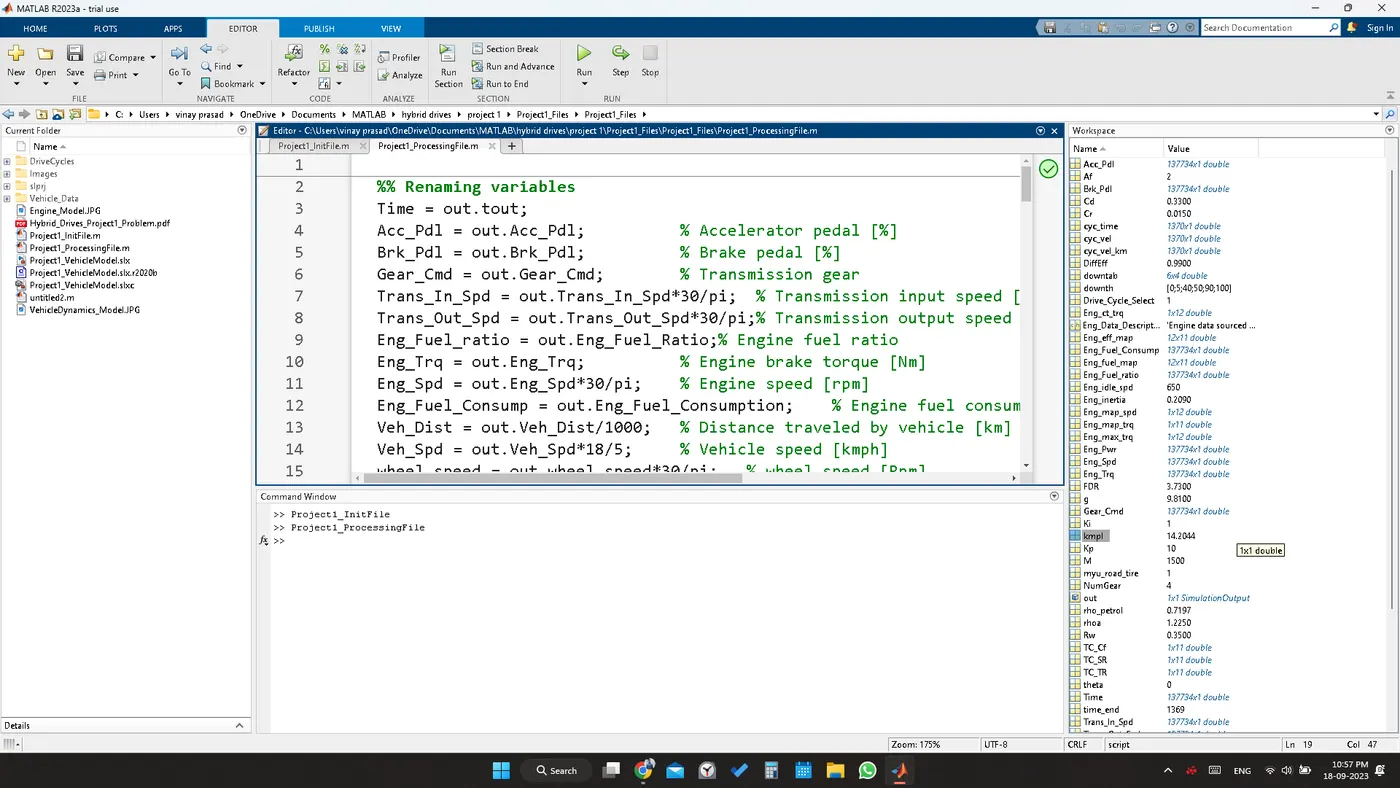
B) plot for the point B
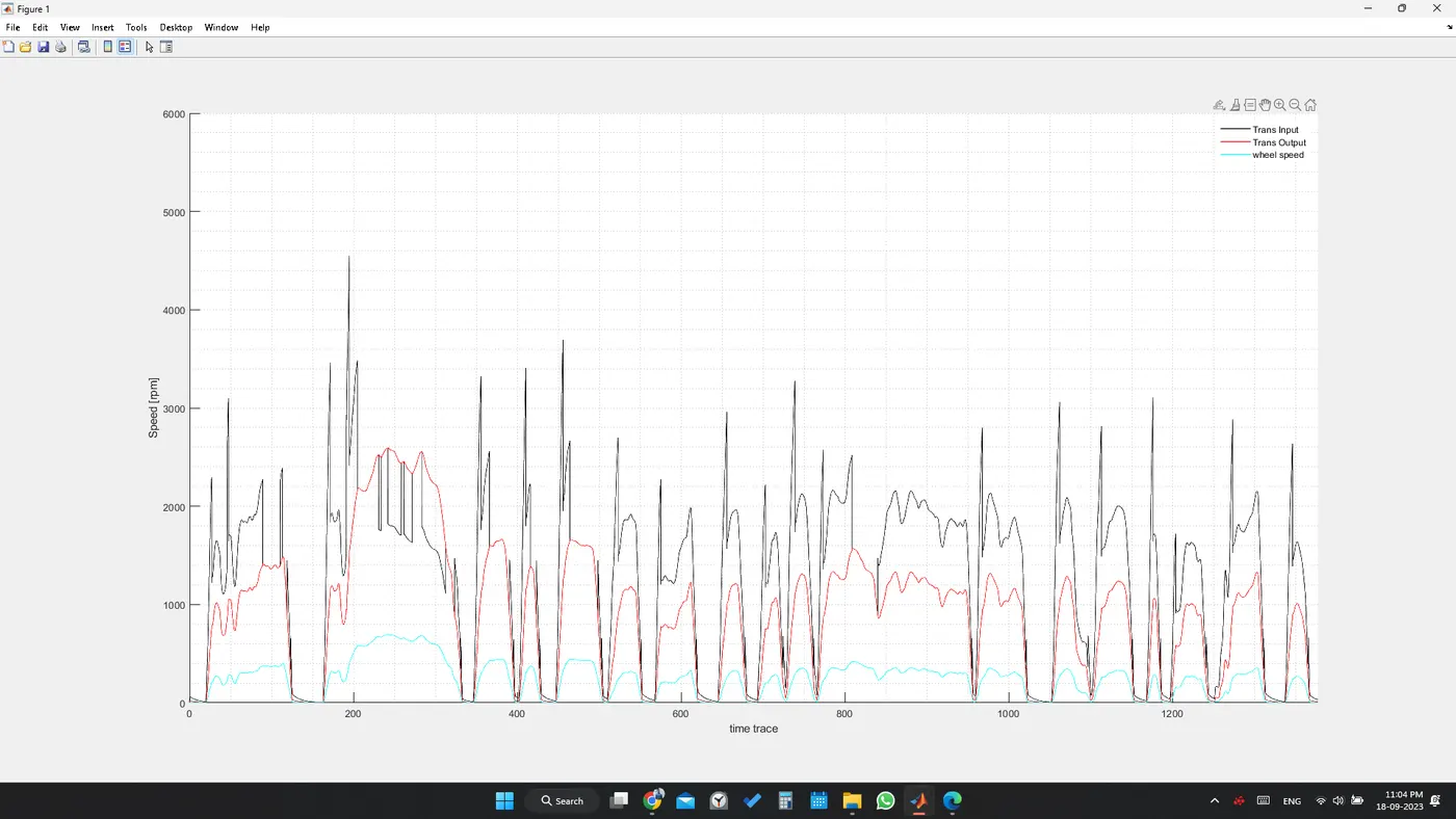
- we can clearly see that the vehicle behaves well in this drive cycle it operates in the required speed and the wheel speed is eventually low as there are many gear ratios in between.
- the automatic transmission used in this engine in the UDDS Drive cycle is able to deliver torque and speed in an efficient manner by shifting the gears in a sequential manner.
C) plot using a subplot for point C
<!-- [if gte vml 1]>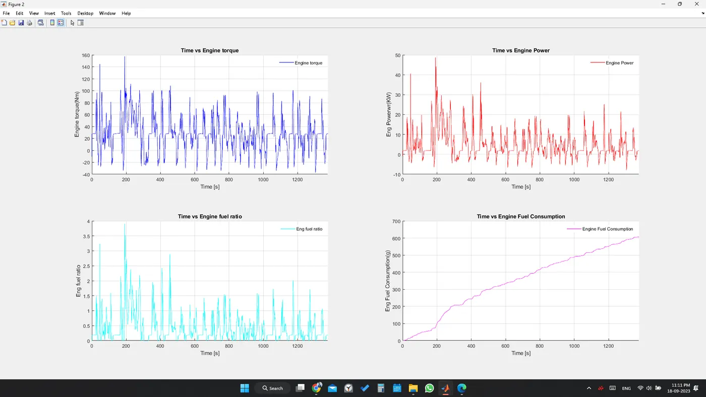 <!--[endif]-->
- we can observe that the engine is producing a good amount of torque to nearly hitting 160 nm of torque at maximum and nearly produces an adequate amount of torque throughout the UDDS drive cycle.
- this vehicle behaved well throughout the UDDS drive cycle delivering required amount of power and torque to the wheels
- the top right plot shows the time vs the engine power plot where the engine is able to provide nearly 50 Kw power wrt time which is good and the power curve seems to meet the specified drive cycle requirements.
- the engine fuel rate curve went up only when there is a requirement of more power which is good and more practical.
- the engine fuel consumption curve went up and up because the fuel consumption will only increase and never decrease w.r.t time and the vehicle returned a fuel economy of 14.2044 per litre of gasoline..
D) Plot using subplot for the point D
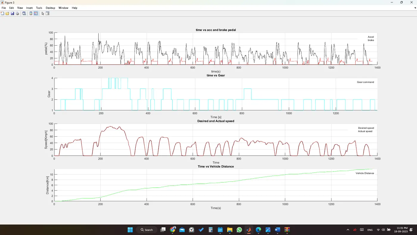
The Plot of acceleration and braking seem to has more amount of acceleration and less amount of braking and the energy is wasted in the form of heat in this drive cycle.
<!-- [if !supportLists]-->· <!--[endif]-->The transmission shift control is able to shift gears frequently according to the requirement of drive cycle, the vehicle barely reached 4 gear very few times as most of it is operating in the lower speeds.
<!-- [if !supportLists]-->· <!--[endif]-->Thanks to the accuracy of the model the vehicle behaved well in the drive cycle by following the drive cycle speed exactly from the starting to the end of the cycle.
<!-- [if !supportLists]-->· <!--[endif]-->The vehicle has crossed more than 10+ km distance by the time of end of drive cycle .
E) Plotting the engine operating points on the engine fuel map.
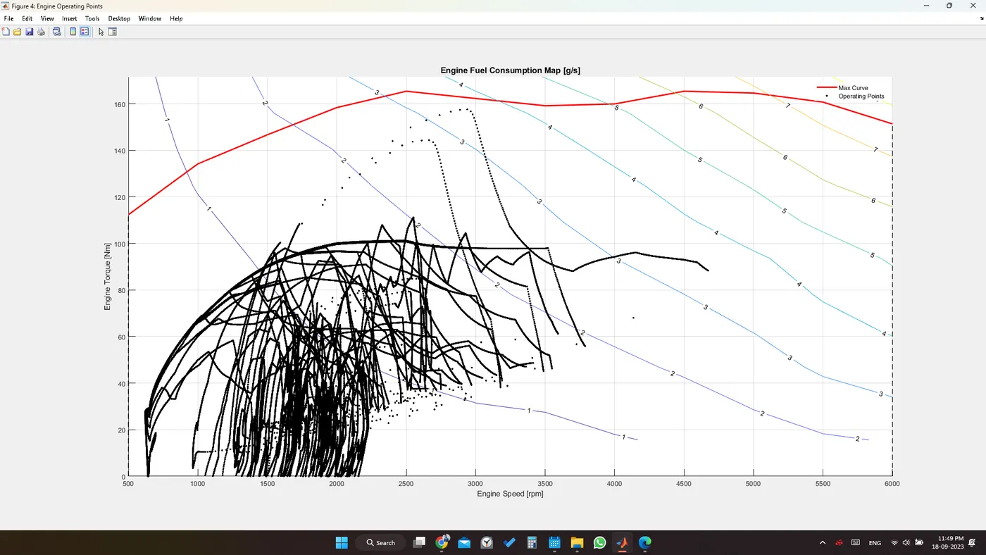
- .The engine operating points are plotted on the engine efficiency map and the engine performed very well in the UDDS Drive cycle
- The operating conditions seems to be in the low rpm sidewhere the transmission and the ECU and every component in the model are performing very well
- the vehicle is able to shift gears in order to operate the engine in lower rpm's which is good for achieving good fuel economy numbers.
- Finally the vehicle behaves stable wrt the drive cycle in every norm as the plot for the desired and actual speed coincide with each other.
THE RESULTS FOR THE UDDS DRIVE CYCLE END HERE
RESULTS FOR THE HWFET DRIVE CYCLE:
- the script (project!_InitFile) is run by changing the drive cycle to '2' i.e (Project1_VehicleModel.slx) was built and the model is run for 2000 sec by adding required to workspace blocks to it .
- the script(Project1_ProcessingFile.m) is run and the required plots are generated.
- This cycle operates for 766 sec's
A) Tabulating the fuel economy numbers (kmpl) for UDDS drive cycle
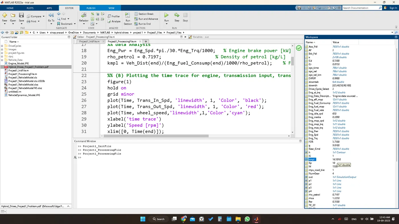
the result obtained using the calculation kmpl = Veh_Dist(end)/(Eng_Fuel_Consump(end)/1000/rho_petrol); is 16.5010
when operated in this drive cycle the vehicle returned a greater mileage as the vehicle did not brake much as it continued in motion from start to the end.
 <!--[endif]-->
B) plot for the point B:
<!-- [if gte vml 1]>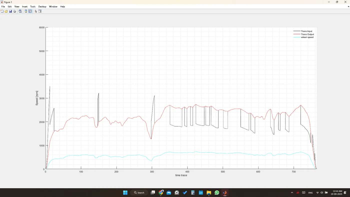 <!--[endif]-->
- we can clearly see that the vehicle behaves well in this drive cycle it operates in the required speed and the wheel speed is eventually low as there are many gear ratios in between.
- the automatic transmission used in this engine in the UDDS Drive cycle is able to deliver the torque and speed in an efficient manner providing the enough push by shifting the gears in a sequential manner.
C) plot using a subplot for point C :
<!-- [if gte vml 1]>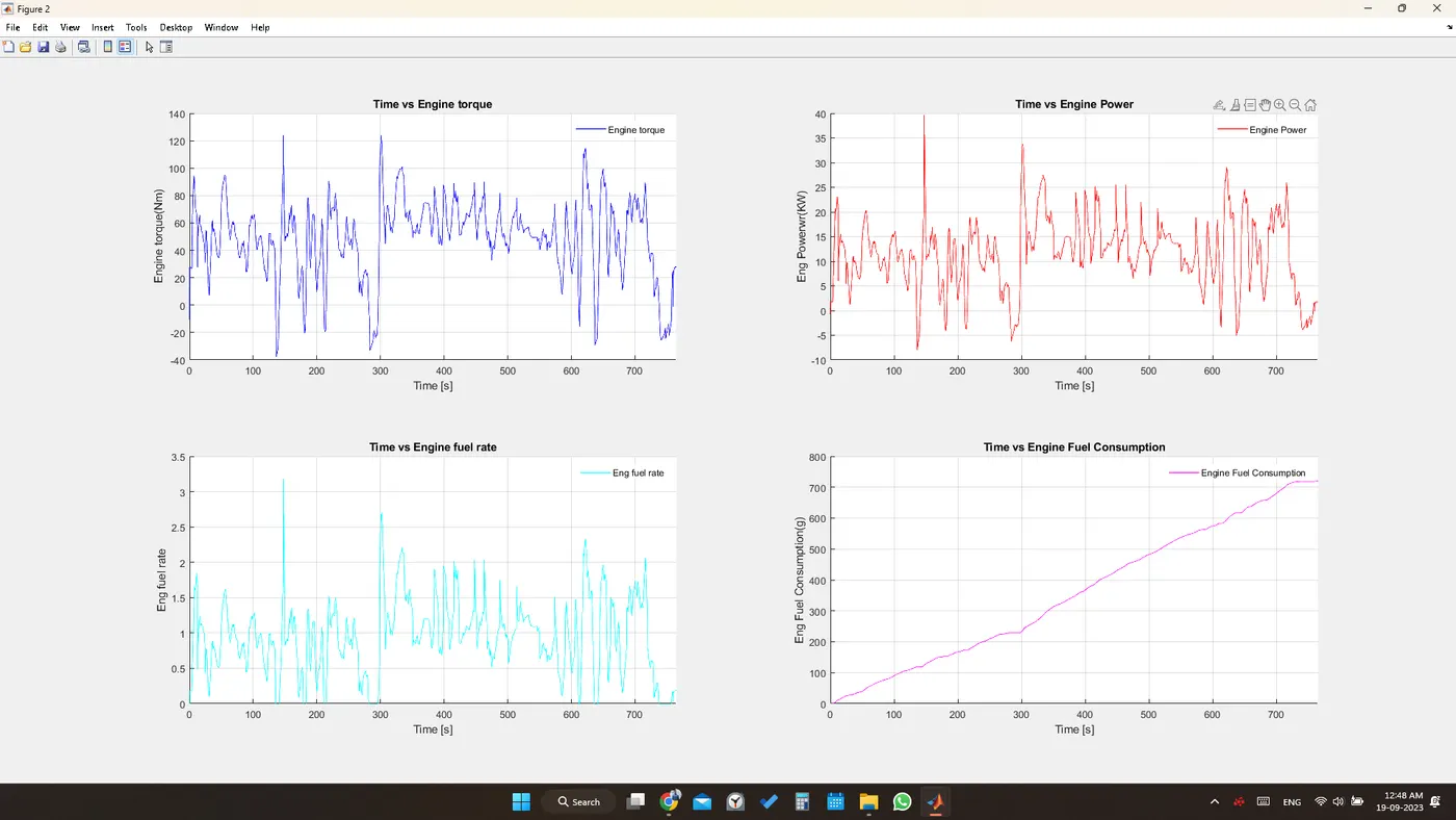 <!--[endif]-->
- we can observe that the engine is producing a good amount of torque to nearly hitting 120 nm of torque at maximum and nearly produces an adequate amount of torque throughout the HWFET drive cycle.
- this vehicle behaved well throughout the HWFET drive cycle delivering required amount of power and torque to the wheels
- the top right plot shows the time vs the engine power plot where the engine is able to provide nearly produce 40 Kw power wrt time which is good and the power curve seems to meet the specified drive cycle requirements.
- the engine fuel rate curve went up only when there is a requirement of more power which is good and more practical and the vehicle returned good mileage in this drive cycle.
- the engine fuel consumption curve went up and up because the fuel consumption will only increase and never decrease w.r.t time and the vehicle returned a fuel economy of 16.5010 per litre of gasoline.
D) Plot using subplot for the point D
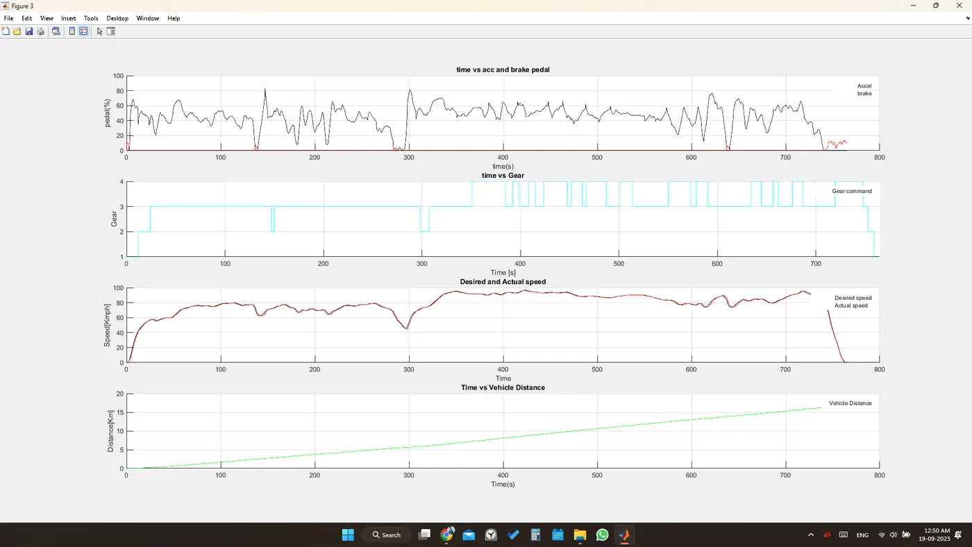
<!-- [if !supportLists]-->· <!--[endif]-->the plot of accelartion and braking seem to have no curve for braking because less amount of friction braking is used in this drive cycle.
<!-- [if !supportLists]-->· <!--[endif]-->The transmission shift control is able to shift gears frequently according to the requirement of drive cycle ranging from (1-4).
<!-- [if !supportLists]-->· <!--[endif]-->Thanks to the accuracy of the model the vehicle behaved well in the drive cycle by following the drive cycle speed exactly.
<!-- [if !supportLists]-->· <!--[endif]-->The vehicle has crossed more than 15 km distance by the time of end of drive cycle.
E) Plotting the engine operating points on the engine fuel map.
<!-- [if gte vml 1]>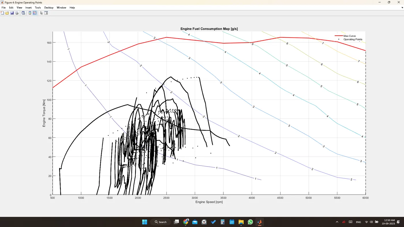 <!--[endif]-->
- .The engine operating points are plotted on the engine efficiency map and the engine performed very well in the HWFET Drive cycle
- The operating conditions seem to be in the low rpm side where the transmission the ECU and every component in the model are performing very well
- the vehicle is able to shift gears in order to operate the engine in lower rpm which is good for achieving good fuel economy numbers.
- Finally, the vehicle operates stable with the drive cycle in every norm as the plot for the desired and actual speeds coincide with each other.
The results for HWFET drive cycle have ended
<!-- [if !supportLineBreakNewLine]-->
<!--[endif]-->
THANKING YOU SIR/MAM
NAGISETTY.VINAY PRASAD