Program to solve otto cycle to create a PV diagram and to find thermal efficiency of engine using MATLAB

Otto cycle - It is a thermodynamic cycle that describes the functioning of a spark ignition piston engine.It describes changes in mass of gas when it is subjected to change in pressure,temperature,volume,heat addition and heat rejection.

It consist of four process or we can say it consists of four states:

State 1-2: Isentropic compression

State 2-3: Constant volume heat addition

State 3-4: Isentropic expansion

State 4-1: Constant volume heat rejection

Formulae used:

where P = pressure of ideal gas

V = volume of ideal gas

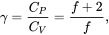
where _{`Cp` = specific heat at constant pressure}

_{CV= specific heat at constant volume}

_{PV/T = constant}

_{Gas equation for ideal gases}

`V/(Vc)=1+1/2(CR-1)[R+1-Cos(theta)-(\sqrt(R^2-(sin(theta)^2)))]`

here V= volume of gas during compression or expansion

Vc = clearance volume of gas

cr = compression ratio

R = cr/a, where a = crank pin radius

thermal efficiency = `eta = 1 - 1/(CR^(gamma-1))`

A fuction called as engine_kinematics is used in the program to call the engine parameters such as bore,stroke,connecting rod and compression ratio whenever needed.

Function Code:

function [V] = engine_kinematics(bore,stroke,con_rod,cr,start_angle,end_angle)
 a = stroke/2;
 R = con_rod/a;
 
v_swept = (pi/4)*bore^2*stroke;
v_clearance = v_swept/(cr-1);
 
 theta = linspace(start_angle,end_angle,180)
 
term1 = 0.5*(cr-1);
term2 = R + 1 - cosd(theta);
term3 = (R^2 - sind(theta).^2).^0.5;

V = (1 + term1*(term2 - term3)).*v_clearance;


end

Main code:

%Program to create a PV diagram of otto cycle and to find the thermal efficiency 

clear all;
close all;
clc;

k = 1.4 %k represents gamma

%parameters at state 1 
p1 = 101325 % in pascal  %assumed to be given
t1 = 500  % in kelvin   %assumed to be given

%engine parameters
bore = 0.1     %width of piston
stroke = 0.1   %length to which piston moves inside cylinder
con_rod = 0.15   %connecting rod length
cr = 12  %compression ratio

v_swept = (pi/4)*bore^2*stroke;
v_clearance = v_swept/(cr-1);
v1 = v_swept + v_clearance  %volume at state 1
v2 = v_clearance    %volume at state 2
 
%parameters at state 2
p2 = p1*cr^k;   %pressure at state 2
t2 = (t1*(p2*v2))/(p1*v1);   %temperature at state 2

%During compression
constant_c = p1*v1^k
V_compression = engine_kinematics(bore,stroke,con_rod,cr,180,0)
P_compression = constant_c./(V_compression.^k)


%parameters at state 3
t3 = 2000   %temperature in kelvin  %assumed to be given
v3 = v2     %volume at state 3
p3 = (p2*t3)/t2;  %pressure at state 3


%During expansion 
constant_c= p3*v3^k
V_expansion = engine_kinematics(bore,stroke,con_rod,cr,0,180)
P_expansion = constant_c./(V_expansion.^k)

%parameters at state 4
v4 = v1    %volume at state 4
p4 = p3*(v3/v4)^k   %pressure at state 4
 


figure(1)
hold on
plot(v1,p1,'*','color','r');
plot(v2,p2,'*','color','g');
plot(v3,p3,'*','color','y');
plot(v4,p4,'*','color','b');
plot(V_compression,P_compression,'linewidth',2,'color','r');
plot([v2 v3],[p2 p3],'linewidth',2,'color','g');
plot(V_expansion,P_expansion,'linewidth',2,'color','y');
plot([v4 v1],[p4 p1],'linewidth',2,'color','b');
legend('p1_v1','p2_v2','p3_v3','p4_v4','Adiabatic compression','Constant volume heat addition','Adiabatic expansion','Constant Vol. heat rejection')
xlabel('V')
ylabel('P')
title("P-V Diagram for otto cycle")


%Thermal efficiency of an internal combustion engine
thermal_efficiency = [1-(1/(cr^(k-1)))]*100;

Output :

P-V curve

Thermal efficiency: