Prandtl Meyer Expansion wave Problem using Converge CFD

Introduction :

In this project, a Prandtl meyer expansion fan is simulated using Converge CFD package and its expansion fan phenomenon is captured. The shock region of the expansion fan is refined using adaptive mesh refinement - Subgrid scale (SGS) criterion. The expansion wave is studied for different sgs parameter & difference in the results and its precision is noted. The shock wave and shock flow boundary conditions are explored in the literature & supersonic flow case setup is explained.

Prandtl Meyer Expansion wave :

A supersonic expansion fan, technically known as Prandtl–Meyer expansion fan, a two-dimensional simple wave, is a centered expansion process that occurs when a supersonic flow turns around a convex corner. The fan consists of an infinite number of Mach Waves, diverging from a sharp corner.

Across the expansion fan, the flow accelerates (velocity increases) and the mach number increases, while the static pressure, temperature & density decrease. Since the process is isentropic, the stagnation properties (e.g. the total pressure and total temperature) remain constant across the fan.

More details & numerical explanation can be found in any Standard FM textbooks & CFD text book like Introduction to CFD by John D anderson.

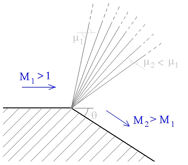
Shock Wave :

A shock wave can be defined as an object which moves faster than the information about it can travel into the surrounding fluid. The fluid near the shock cannot react before it arrives and the properties like density, pressure, temperature, velocity & mach number of the fluid changes almost instantanously.

Shock waves occur when the object moves faster than the speed of sound and also when there is an abrupt decrease or increase in flow area. The changes in the flow properties are irreversible and entropy of entire system increases by law of thermodynamics.

Shock waves are researched for supersonic flights & atmospheric reentry of space vehicles & it has usage nowadays in many medical fields and artificial world as well.

Shock Flow Boundary conditions :

1. Dirichlet Boundary condition: This condition specifies the value that the unknown function needs to take on along the boundary of the domain
2. Neumann boundary condition : It specifies the values that the derivative of a solution is going to take on the boundary of the domain.
3. Robin Boundary condition : It consists of a linear combination of the values of the field and its derivatives on the boundary
4. Mixed Boundary condition : It consists of applying different types of boundary conditions in different parts of the domain. It is important to notice that boundary conditions must be applied on the whole boundary: the “free” boundary is anyways subjected to a homogeneous Neumann condition. The mixed boundary condition differs from the Robin condition because the latter consists of different types of boundary conditions applied to the same region of the boundary, while the mixed condition implies different types of b.c. applied to different parts of the boundary.

These are certain boundary conditions used, for capturing shocks generally when the flow is supersonic since the inlet velocity provided in inlet of this project is double the sound velocity, the flow quantities like pressure, density etc are extrapolated from the interior. As mentioned above during shocks the flow properties changes instantaneously, there is noway to predict the outflow conditions except for maybe certain well experimented and highly controlled shock problems. Hence for shock flows inlet conditions are specified like in this case, velocity, temperature & pressure i.e Dirichlet Bc and outflow is set to Zero gradient i.e Neumann Boundary condition which makes this case a Mixed BC problem.

Geometry in Converge Studio :

The geometry is created in CAD software and Stl file imported in Converge studio. Converge automatically triangulates the entire geometry. On the side view of the image you can more clearly see the convex bent after a straight path in the geometry. The boundary is flagged as inlet at the pink region and outlet at is opposite and the side walls are treated as 2D boundary. More details given in case setup.

Meshing :

Adaptive Mesh Refinement is a method of adapting the accuracy of a solution within certain sensitive or turbulent regions of simulation, dynamically and during the time the solution is being calculated. When solutions are calculated numerically, they are often limited to pre-determined quantified grids as in the Cartesian plane which constitute the computational grid, or 'mesh'

In this Project, Subgrid scale Amr is used on the Temperature field of the Simulation . Two different subgrid criteria are simulated - one with sgs 0.05 & another sgs 0.01, the results are presented ahead. So converge calculates the second order temperature field and while calculating if the difference is above say 0.05k it will perform a refinement of the cells with embedding of 2 as provided.

The formula used is :

With mesh size 0.8 m the first embedding gives the grid side of 0.4 m & second embedding gives 0.2 m grid size.

Case 1 : with AMR SGS 0.05 : (final mesh shown)

Mesh size : 0.8 m in xyz direction. The area around the refine zone is the base mesh and the whole domain initially looks like it.

Case 2 : with AMR SGS 0.01 : (final mesh shown)

Mesh size : 0.8 m in xyz direction

The smaller elements seen in the mesh are the refined zones after the detecting the temperature subgrid criteria it performs amr.

Mesh Cell count :

The adaptive mesh refinement cell counts is shown, the curve denotes how the mesh has been refined and in the y axis the total cells during that particular cycle is presented. The refinement was nearly 3 times more about 17000 in sgs 0.01 criteria from the sgs 0.05 with count nearly 7800.

Case Setup :

1. Application type : Time Based

2. Material : Air mixture ( Gas simulation)

3. Gas Species : 02 , N2 .

4. Solver : Steady state solver , Fully Hydrodynamic.

5. Gas flow solver : Compressible.

6. Misc : Momentum , Energy on

7. Steady state monitor : On. - min cycles : 500

8. Monitor Variables : AVG TEMP & AVG DENSITY at Outlet

9. Simulation Time parameters :

i. Start 0 cyc

ii. End : 25000 cyc.

iii. Initial Time-step : 1e-9s

iv. minimum Time-step 1e-9s

v. Max time-step 1s.

10. Solver scheme : Piso algorithm : Density Based

11. Boundary Conditions :

i. Inlet : Inflow ; velocity (x) :680 m/s ;Temp : 286.1 k ; Species : O2 , N2.

ii. Outlet : Zero Normal Gradient ; Species : O2, N2.

iii. Front & Back : Two_D

iv. Top-bottom-wall: Stationary fixed : Slip

12. Regions & Initialization :

13 Region 0 created : Velocity X dir - 680 m/s ; Pressure 50000 pa ; Temp : 286.1 K ; Species : O2,N2 .

14. Turbulence Model : RNG K-epsilon

15. Output Files : Time interval for writing 3D output data files : 250 cyc.

16. Max restart files saved : 3

17. Turbulence Model :RNG k-epsilon

18. Grid control : As mentioned in Meshing.

Solution & Post Processing :

The results are post processed in Paraview software.

Case 1 : With AMR SGS 0.05

Temperature Contour :

Tthe animation shown below displays the physics captured on the expansion fan as shown in the diagram in the Introduction part above. This expansion fan as you can see was fanning out very wide as it is supersonic flow region but infact it was going out of its practical solution if not for AMR. The amr continously refined the Temperature region and the solution fan was contained and accurately captured.

Temperature Plot :

Pressure Contour :

As the temperature varies similarly other flow properties also varies in the expansion fan. The pressure contour is shown. Above the fan the pressure is high and it goes on decreasing as it approaches below the shap expansion fan.

Pressure Plot : Similarly at outlet bound id 2 the Static pressure decreases.

Velocity Contour :

Mach Number Plot :

The mach No. at bound id 1 i.e. inlet is 2 and it increases towads the outlet and reaches near 2.14 at bound id 2 outlet.

Density Plot : Density of decreases towards outlet.

Case 2: With AMR SGS 0.01

Temperature Contour : With Mesh

We can see more refined solution and more nicer looking contour towards the end of the fan and along its edges, it has happened due to more stricter sgs criterion. It is understood that as the sgs will be reduced we can expect a more refined solution with increase in mesh sizes and better result. The results are nearly same with sgs 0.05 for this problem because its a simple problem so we can conclude our solution is Grid independent.

Without Mesh

Similarly the other results of the problem like plots and contours doesnt vary & are similar and its physics is same hence its understood and isnt shown here.

------------------------------------------- THE END -----------------------------------------------------------