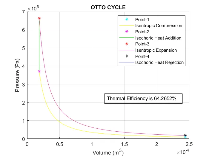
Plotting the P-V diagram of the Otto cycle and to find the thermal efficiency of the Otto cycle
Definition of Otto cycle:
The Otto cycle is a thermodynamic cycle that is commonly used in all spark ignition engines (i.e is petrol engines - 2-stroke or 4-stroke). In a four-stroke engine, there are typically four strokes which are named as;
1) Intake stroke
2) Compression stroke
3) Power stroke
4) Expansion stroke
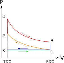
Process (0-1) - Intake stroke:
In this stroke, at constant pressure, the air enters the engine. Here the piston moves from TDC to BDC, here the inlet valve is opened and the exhaust valve will be closed.
Process (1-2) - Compression stroke (Isentropic compression):
In this stroke, the air in the cylinder is compressed adiabatically. Here the piston moves from BDC to TDC, while the inlet valve and the exhaust valve will remain closed.
Process (2-3) - Combustion (Constant volume heat addition):
In this process, at constant volume heat is added, i.e the air-fuel mixture is ignited by a spark plug for rapid combustion of the air-fuel mixture. The inlet valve and the exhaust valve will remain closed.
Process (3-4) - Power stroke (Isentropic expansion):
In this stroke, the air in the cylinder is expanded adiabatically, due to the rapid ignition of the air-fuel mixture a force is exerted on the piston. Therefore the piston moves from TDC to BDC, while the inlet valve and the exhaust valve will remain closed.
Process (4-1) - Constant volume heat rejection:
In this process, at constant volume heat is rejected from the air. The inlet valve and the exhaust valve will remain closed.
Process (1-0) - Exhaust stroke:
In this stroke, the air in the cylinder is pushed out of the cylinder by the piston, which is called exhaust gas. Therefore the piston moves from BDC to TDC, while the inlet valve will remain closed, but the exhaust valve will be opened.
This is the complete cycle of a four-stroke Otto cycle, This cycle is performed again and again for the continuous operation of the engine.
1) This is the main code for plotting the P-V diagram of the Otto cycle:
% To create a P-V diagram of the otto cycle and to find the efficiency of the engine

close all
clear all
clc

%% Inputs required for the calculation of P-V diagram for otto cycle

gamma = 1.4

%Engine geometric parameters

bore = 0.076;      %Bore diameter
stroke = 0.0496;   %Stroke length
conn_rod = 0.11;   %Connecting rod length

%compression ratio = v1/v2 = (v_swept + v_clearance)/ v_clearance
cr = 13.1;

%State variables at point 1

p1 = 101325
t1 = 500

%Maximum temperature that should be attained by the engine

t3 = 2500

%With the engine geometric parameters we can calculate the other state variables

%Swept volume is the volume of the engine cylinder
v_swept = (pi/4)*bore^2*stroke;

%Clearancee volume is the volume between the cylinder head and the piston when the piston is at TDC
v_clearance = v_swept/(cr-1);

%Volume at state 1, i.e when the piston is at BDC
v1 = v_swept + v_clearance

%Volume at state 2, i.e when the piston is at TDC
v2 = v_clearance

%% Process 1-2: Isentropic compression

%p*v^gamma = constant
%p1v1^gamma = p2v2^gamma
%p2 = p1 * (v1 / v2)^gamma
%cr = v1/v2

p2 = p1*cr^gamma;

%As per Ideal gas gas law
%pv/t = constant
%p1v1/t1 = p2v2/t2

t2 = p2*v2*t1/(p1*v1);

constant_c1 = p1*v1^gamma;
v_compression = engine_kinematics(bore,stroke,conn_rod,cr,180,0);

p_compression = constant_c1./v_compression.^gamma;

%% Process 2-3: Constant volume heat addition

%Since it is a contant volume process,

v3 = v2

%As per Ideal gas gas law
%pv/t = constant
%p3v3/t3 = p2v2/t2
%here v2 = v3

p3 = (p2*t3)/t2;

%% Process 3-4: Isentropic Expansion

%At the end of this process the piston would reach BDC
%volume at points 4 and 1 are same

v4 = v1

%p*v^gamma = constant
%p3v3^gamma = p4v4^gamma
%p4 = p3 * (v3 / v4)^gamma

p4 = p3*(v3/v4)^gamma


constant_c2 = p3*v3^gamma;
v_expansion = engine_kinematics(bore,stroke,conn_rod,cr,0,180);

p_expansion = constant_c2./v_expansion.^gamma;

%% Process 4-1: Constant volume heat rejection

%% Thermal Efficiency of the Engine

%The thermal efficiency of the engine is derived from the equation below
thermal_efficiency = (1 - (1/cr^(gamma-1)))*100

%% Plotting P-V diagram of Otto cycle

figure('name','P-V Diagram of Otto cycle','numbertitle','off')

hold on
grid on

xlabel('Volume (m^3)')
ylabel('Pressure (Pa)')

title('OTTO CYCLE')

%Plotting the state points;
plot(v1,p1,'*','color','cyan')
plot(v_compression,p_compression,'color','yellow')
plot(v2,p2,'*','color','magenta')
plot([v2,v3],[p2,p3],'color','green')
plot(v3,p3,'*','color','red')
plot(v_expansion,p_expansion,'color','[0.9,0.25,0.6]')
plot(v4,p4,'*','color','black')
plot([v4,v1],[p4,p1],'color','blue')

%Legends are used to name the curve
legend('Point-1','Isentropic Compression','Point-2','Isochoric Heat Addition','Point-3','Isentropic Expansion','Point-4','Isochoric Heat Rejection')

%By creating a textbox annotation we can display the efficiency value in the same plot figure
annotation('textbox', [0.5, 0.3, 0.1, 0.1],'string',"Thermal Efficiency is "+thermal_efficiency+"%")

%% Result

% The Matlab program is successfully compiled and the P-V diagram is plotted for the Otto cycle
% The thermal efficiency of the engine is also shown in the same graph using annotations
2) Subfunction for obtaining the path traced by the isentropic process:
%Function to trace the path of an isentropic process

function [v] = engine_kinematics(bore, stroke, con_rod, cr, start_angle, end_angle)

%Crank pin radius is half of stroke
a = stroke/2

%Ratio of connecting rod length and crankpin radius
R = con_rod/a

%swept volume
v_s = pi/4*bore^2*stroke;

%compression volume
v_c = v_s/(cr-1);

%crank angle
theta = linspace(start_angle,end_angle,200);

%Change in volume inside the combustion chamber is given by the equation
%(v/v_c) = 1+ 0.5(cr - 1)(R+1-cos(theta)-(R^2-sin(theta)^2)^0.5)

%splitting the above equation into separate terms

term1 = 0.5*(cr-1);
term2 = R +1 - cosd(theta);
term3 = (R^2 - sind(theta).^2).^0.5;

v = (1 + term1*(term2 - term3)).*v_c;

end
Errors faced and solution to overcome those errors:
1) When using the text command to show the efficiency value on the graph, there were some issues with the plot command. Therefore textbox feature in the annotation command is used to display the efficiency value in the figure, where the graph is plotted for better understanding.
2) In the annotation command to display the percentage symbol, it was given between " % " (double quotes). If this symbol was not given in between double quotes then any characters used after the % symbol will be considered as comments.
Output: