p-V Diagram of an Otto cycle using MATLAB
Aim:
The main aim is to create a p-V Diagram of an Otto cycle and to calculate it’s Thermal Efficiency.
Equations used:
- Relation between crank angle and Volume in the Combustion chamber:
`V/V_c =1+ 1/2(r_c-1)[R+1-cosθ- (R^2-sin^2θ)^(1/2)]`
Where,
V = Compression or Expansion Volume
`V_c`= Clearance Volume
`r_c` = Compression ratio
R = Crankpin Radius
`theta`= Crank Angle
- Swept Volume (`V_s`):
The swept volume is the volume of air displaced by the diameter of the piston in one full stroke from the Bottom Dead Centre (BDC) to the Top Dead Centre (TDC).
`V_s=π/4×("Bore")^2×Stroke`
Where,
Bore = Diameter of each cylinder.
Stroke = Length that travels when moving from the bottom position to the top position.
- Clearance Volume (`V_c`):
Clearance Volume is the volume between the cylinder head and the piston top when the piston is at the Top Dead Centre (TDC).
(Or)
The volume of the Cylinder that is not swept by the piston is called the Clearance Volume.
`V_c=V_s/((r_c-1))`
- Reversible Adiabatic process:
`P×V^γ=C`
Where,
P = Pressure
V = Volume
`γ=C_p/C_v` (`C_p`= specific heat for constant pressure; `C_v`= Specific heat for constant volume)
- Ideal gas law:
`PV=nRT`
Where,
P = Pressure of the Gas
V= Volume of the Gas
n = Amount of Substances/ Number of moles.
R = Ideal or Universal Gas Constant
T = Absolute Temperature of the gas
- Efficiency of the Engine:
`η=1-1/r_c^((γ-1))`
or
`η=1-((T_4-T_1)/(T_3-T_2))`
Where,
η = Thermal Efficiency of the Engine.
Working Principle:
- An Otto cycle is an idealized thermodynamic cycle that describes the functioning of a typical spark ignition piston engine.
- It is the thermodynamic cycle most commonly found in automobile engines.
- The internal combustion engine working on the principle of the Otto cycle is called Spark Ignition (SI) engine in which used gasoline as the fuel.
- The four strokes of the Otto cycle or four-stroke engine are suction of fuel, compression of fuel, combustion, expansion of fuel, and exhaust of burnt fuel.
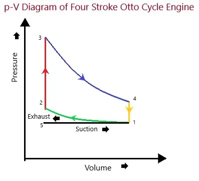
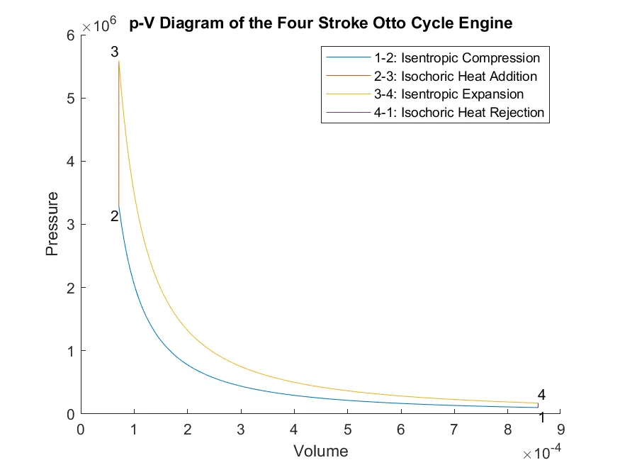
1-2: Reversible Adiabatic (Isentropic) Compression
2-3: Constant Volume (Isochoric) Heat Addition
3-4: Isentropic Expansion
4-1: Isochoric Heat Rejection
- Suction Stroke: During this stroke, the piston moves from Top Dead Centre (TDC) to the Bottom Dead Centre (BDC). The inlet valve opens and the appropriate air-fuel mixture is sucked into the cylinder. The exhaust valves remain closed during this stroke.
- Compression Stroke: In this Stroke, the piston moves from 1-2 towards TDC and compresses the mixture drawn from suction stroke. The pressure of the mixture increases. Just before the end of the stroke, the spark plug initiates a spark that ignites the mixture and combustion takes place at Constant Volume (2-3). During this stroke both the valves remain closed.
- Expansion Stroke: When the mixture is ignited the hot gases are produced which move the piston from TDC to BDC and the work is obtained in this stroke while the other 3 strokes remain idle. The expansion of gases is shown in 3-4. Both the valves are closed initially but when the piston reaches BDC the exhaust valve opens
- Exhaust Stroke: Here the gases from which the work has been collected become useless after completion of a previous stroke. In 4-1, they are made to escape through the exhaust valve to the atmosphere. The piston moves from BDC to TDC and the exhaust gases are taken out of the engine. This is represented by the line (1-5).
Procedure:
- Initially, the code requires some input values which can either be inserted directly or it can either be inserted using the input () function. Some of the directly inserted inputs are as follows.
Adiabatic Index(`gamma`)= 1.4
Pressure at Point 1 (`p_1`)= 101325 pa (1atm =101325 Pa),
Temperature at point 1 (`T_1`)= 500 K
Temperature at point 3 (`T_3`)= 2300 K
%Inputs
gamma = 1.4;

% State Variables (p,t,v are pressure,temperature and Volume and 1,2,3,4
% are at different states)
p1 = 101325;
t1 = 500;
t3 = 2300;
% Engine Geometric Parameters
bore = input('Enter the Bore value in meters(m): ');                % Bore in Meters
stroke = input(' Enter the Stroke value in meters(m): ');           % Stroke in Meters
con_rod = input('Enter the Connecting rod value in meters(m): ');   % Connecting Rod in Meters
cr = input ('Enter the Compression ratio value: '); % Compression Ratio- A function is created to give a relation between crank angle and Volume in the Combustion chamber.
function [V] = engine_kinematics(bore,stroke,con_rod,cr, start_crank, end_crank)

a= stroke/2;
R= con_rod/a;
v_s = pi/4*bore^2*stroke;
v_c= v_s/(cr-1);

theta = linspace(start_crank, end_crank, 100);
term1= (1/2)*(cr-1);
term2= R +1 - cosd(theta);
term3 = (R^2 - sind(theta).^2).^(1/2);

V= (1+ term1*(term2-term3)).*v_c;
end
- The swept volume and clearance volume is calculated.
% Calculating the swept Volume and the Clearance Volume
v_Swept = (pi/4)*bore^2*stroke;
v_clearance = v_Swept/ (cr-1);

v1 = v_Swept +v_clearance;
v2 = v_clearance;- The State variable at location 1,2,3 and 4 are calculated as explained in the code
% State Variable at state 2
% p2v2^gamma = p1v1^gamma
% p2 = p1*(v1/v2)^gamma= p1*cr^gamma
p2= p1*cr^gamma;

%p1v1/t1 = p2v2/t2 | t2 = p2*v2*t1/(p1*v1)
t2 = p2*v2*t1/(p1*v1);

constant_c = p1*v1^gamma;
V_compression = engine_kinematics(bore,stroke,con_rod,cr,180,0);

P_compression = constant_c./V_compression.^gamma;

% State varabile at state point 3
v3= v2;

%p3v3/t3 = p2v2/t2 | p3 = p2*t3/t2
p3 = p2*t3/t2;

constant_e = p3*v3^gamma;
V_expansion = engine_kinematics(bore,stroke,con_rod,cr,0,180);

P_expansion = constant_e./V_expansion.^gamma;

% State Variable at state point 4
v4=v1;

%p3v3^gamma = p4v4^gamma |p4 = p3 (v3/v4)^gamma
p4 = p3 *(v3/v4)^gamma;

%p4*v4/t4= p1*v1/t1 || t4= (p4/p1)*t1
t4= (p4*t1/p1);- The Thermal Efficiency of the Simple Air standard Otto Cycle is written.
%The Efficiency of an otto cycle is given by the formula:
%efficiency = 1-((t4-t1)/(t3-t2));
efficiency = 1 - 1/ (cr^(gamma-1));
fprintf('The Thermal Efficiency of an Otto Cycle is %d n', efficiency);- The Plotting of the graph is done.
figure(1);
hold on ;

title('p-V Diagram of the Four Stroke Otto Cycle Engine')
xlabel('Volume')
ylabel('Pressure')

% legend('1-2: Isentropic Compression','2-3: Isochoric Heat Addition', '3-4: Isentropic Expansion','4-1: Isochoric Heat Rejection');
plot(V_compression, P_compression);
plot([v2 v3], [p2 p3]);
plot(V_expansion, P_expansion);
plot([v4 v1],[p4 p1]);
legend('1-2: Isentropic Compression','2-3: Isochoric Heat Addition', '3-4: Isentropic Expansion','4-1: Isochoric Heat Rejection');

text( v1 ,p1, '1','HorizontalAlignment', 'left', 'VerticalAlignment', 'Top');
text( v2 ,p2, '2','HorizontalAlignment', 'Right', 'VerticalAlignment', 'Top');
text( v3 ,p3, '3','HorizontalAlignment', 'Right', 'VerticalAlignment', 'Bottom');
text( v4 ,p4, '4','HorizontalAlignment', 'left', 'VerticalAlignment', 'Bottom');
saveas(gcf, 'p-V Diagram of an Simple Air Standard Otto Cycle.png ')
Code:
- For Function:
function [V] = engine_kinematics(bore,stroke,con_rod,cr, start_crank, end_crank)

a= stroke/2;
R= con_rod/a;
v_s = pi/4*bore^2*stroke;
v_c= v_s/(cr-1);

theta = linspace(start_crank, end_crank, 100);
term1= (1/2)*(cr-1);
term2= R +1 - cosd(theta);
term3 = (R^2 - sind(theta).^2).^(1/2);

V= (1+ term1*(term2-term3)).*v_c;
end
- Main Code:
% Plotting the PV Diagram and Calculating the Thermal Efficiency
% 1-2: Reversible Adiabatic (Isentropic) Compression
% 2-3: Constant Volume (Isochoric) Heat Addition
% 3-4: Isentropic Expansion
% 4-1: Isochoric Heat Rejection

clear
close
clc

%Inputs
gamma = 1.4;

% State Variables (p,t,v are pressure,temperature and Volume and 1,2,3,4
% are at different states)
p1 = 101325;
t1 = 500;
t3 = 2300;
% Engine Geometric Parameters
bore = input('Enter the Bore value in meters(m): ');                % Bore in Meters
stroke = input(' Enter the Stroke value in meters(m): ');           % Stroke in Meters
con_rod = input('Enter the Connecting rod value in meters(m): ');   % Connecting Rod in Meters
cr = input ('Enter the Compression ratio value: ');                 % Compression Ratio

% Calculating the swept Volume and the Clearance Volume
v_Swept = (pi/4)*bore^2*stroke;
v_clearance = v_Swept/ (cr-1);

v1 = v_Swept +v_clearance;
v2 = v_clearance;
% State Variable at state 2
% p2v2^gamma = p1v1^gamma
% p2 = p1*(v1/v2)^gamma= p1*cr^gamma
p2= p1*cr^gamma;

%p1v1/t1 = p2v2/t2 | t2 = p2*v2*t1/(p1*v1)
t2 = p2*v2*t1/(p1*v1);

constant_c = p1*v1^gamma;
V_compression = engine_kinematics(bore,stroke,con_rod,cr,180,0);

P_compression = constant_c./V_compression.^gamma;

% State varabile at state point 3
v3= v2;

%p3v3/t3 = p2v2/t2 | p3 = p2*t3/t2
p3 = p2*t3/t2;

constant_e = p3*v3^gamma;
V_expansion = engine_kinematics(bore,stroke,con_rod,cr,0,180);

P_expansion = constant_e./V_expansion.^gamma;

% State Variable at state point 4
v4=v1;

%p3v3^gamma = p4v4^gamma |p4 = p3 (v3/v4)^gamma
p4 = p3 *(v3/v4)^gamma;

%p4*v4/t4= p1*v1/t1 || t4= (p4/p1)*t1
t4= (p4*t1/p1);

%The Efficiency of an otto cycle is given by the formula:
%efficiency = 1-((t4-t1)/(t3-t2));
efficiency = 1 - 1/ (cr^(gamma-1));
fprintf('The Thermal Efficiency of an Otto Cycle is %d n', efficiency);


figure(1);
hold on ;

title('p-V Diagram of the Four Stroke Otto Cycle Engine')
xlabel('Volume')
ylabel('Pressure')

% legend('1-2: Isentropic Compression','2-3: Isochoric Heat Addition', '3-4: Isentropic Expansion','4-1: Isochoric Heat Rejection');
plot(V_compression, P_compression);
plot([v2 v3], [p2 p3]);
plot(V_expansion, P_expansion);
plot([v4 v1],[p4 p1]);
legend('1-2: Isentropic Compression','2-3: Isochoric Heat Addition', '3-4: Isentropic Expansion','4-1: Isochoric Heat Rejection');

text( v1 ,p1, '1','HorizontalAlignment', 'left', 'VerticalAlignment', 'Top');
text( v2 ,p2, '2','HorizontalAlignment', 'Right', 'VerticalAlignment', 'Top');
text( v3 ,p3, '3','HorizontalAlignment', 'Right', 'VerticalAlignment', 'Bottom');
text( v4 ,p4, '4','HorizontalAlignment', 'left', 'VerticalAlignment', 'Bottom');
saveas(gcf, 'p-V Diagram of an Simple Air Standard Otto Cycle.png ')
Result:
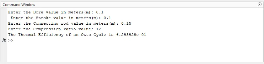
The Thermal Efficiency is calculated and the PV diagram is drawn.
The Thermal Efficiency calculated is 0.6299 i.e. 62.99%.
The p-V Diagram is shown below.