Otto Cycle using PYTHON

Aim : To plot a PV graph for otto cycle and calculating its thermal efficiency.

Theory:

Otto cycle is an idealized thermodynamic cycle that describes the functioning of a typical and most commonly used piston engines.

Piston kinematics can be used to understand the variation of volume and pressure with the crank angle.

The otto cycle basically has four processes which results in the mechanical output of the engine.

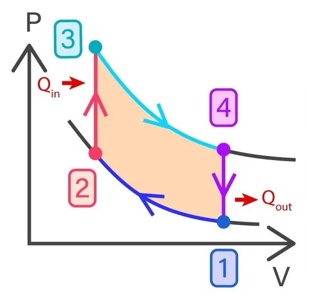
The processes are as follows:

1-2 : Isentropic compression

2-3 : Constant Volume heat addition

3-4 : Isentropic Expansion

4-1 : Constant volume heat rejection

The system is defined to be the mass of air that's drawn from the atmosphere into the cylinder, compressed by the piston, heated by the spark ignition of the added fuel, allowed to expand as it pushes on the piston, and finally exhausted back into the atmosphere. The mass of air is followed as its volume, pressure and temperature change during the various thermodynamic steps. As the piston is capable of moving along the cylinder, the volume of the air changes with its position in the cylinder.

The compression and expansion processes induced on the gas by the movement of the piston are idealised as reversible, i.e., no useful work is lost through turbulence or friction and no heat is transferred to or from the gas during those two processes. Energy is added to the air by the combustion of fuel. Useful work is extracted by the expansion of the gas in the cylinder. After the expansion is completed in the cylinder, the remaining heat is extracted and finally the gas is exhausted to the environment.

Here we'll make use of the below given formula to plot for the expansion and compression processes in the otto cycle by considering engine kinematics.

Pyhton Code for Otto Cycle:

import matplotlib.pyplot as plt 
import math
import numpy as  np 
import scipy

# FOR ENGINE KINEMATICS

def function(bore,stroke,con_rod,cr,crank_start,crank_end):
	
	a = stroke/2
	R = con_rod/a

	v_s = (math.pi/4)*pow(bore,2)*stroke
	v_c = v_s/(cr-1)
	

	sc = math.radians(crank_start)
	ec = math.radians(crank_end)

	num_values = 50
	
	theta = np.linspace(sc,ec,num_values)

	V = []


	for  THETA in theta:
		
		v = R + 1 - math.cos(THETA)-(pow(pow(R,2)-pow(math.sin(THETA),2),0.5))
		V.append(v_c + (v_c*0.5*(cr-1)*v))
	
	return(V)
		
	

#INPUTS

p1 = 101325
t1 = 500
gamma = 1.4

#GEOMETRIC PARAMETERS

bore = 0.1
stroke= 0.1
con_rod = 0.15
cr = 7
t3 =  2300

#VOLUME COMPUTATION

v_s = (math.pi/4)*pow(bore,2)*stroke
v_c = v_s/(cr-1)
v1 = v_s + v_c


#STATE POINT 2

v2 = v_c
p2 = p1*pow(v1,gamma)/pow(v2,gamma)
t2 = (p2*v2*t1)/(p1*v1)


#ISENTROPIC COMPRESSION

const_c = p1*pow(v1,gamma)
v_compression = function(bore,stroke,con_rod,cr,180,0)
p_compression = []

for v in v_compression:
	p_compression.append(const_c/pow(v,gamma))

#STATE POINT 3

v3 = v2
p3 = (p2*v2*t3)/(v3*t2)


#ISENTROPIC EXPANSION

const_c = p3*pow(v3,gamma)
p_expansion = []
v_expansion = function(bore,stroke,con_rod,cr,0,180)

for v in v_expansion:
	p_expansion.append(const_c/pow(v,gamma))


#STATE POINT 4

v4 = v1
p4  = p3*pow(v3,gamma)/pow(v4,gamma)
t4 = (p4*v4*t3)/(p3*v3)


#PLOTTING

plt.figure()
plt.plot(v_compression,p_compression,label='Isentropic Compression')
plt.plot([v2,v3],[p2,p3],label='Constant Volume heat addition')
plt.plot(v_expansion,p_expansion,label='Isentropic Expansion')
plt.plot([v4,v1],[p4,p1],label='Constant Volume heat rejection')
plt.xlabel('Volume')
plt.ylabel('Pressure')
plt.legend()
plt.show()

#THERMAL EFFICIENCY

n = 1 - 1/pow(cr,gamma-1)
n = str(n)
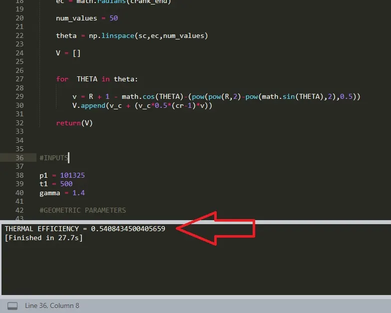
print('THERMAL EFFICIENCY = ' + n)

Outputs:

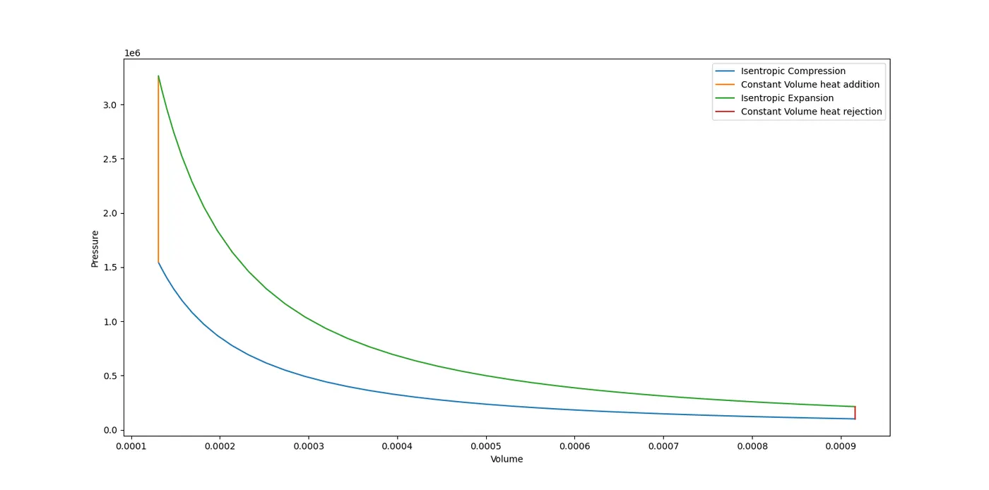
(1) PV Diagram :

(2) Thermal Efficiency :