Otto cycle
AIM-
To plot the Air Standard Cycle (Otto cycle) of a 4 stroke engine.
Objective-
- 1. To plot the P-V plot for an Otto cycle for a 4 stroke engine.
- To find the Thermal efficiency of the engine.
Introduction-
Otto cycle is the basic Air cycle that provides help in understanding how a 4 stroke engine work. In the Automobile industry, the efficiency of the engine is a great concern as the fuel consumption increases if the efficiency or thermal efficiency decreases.
So, this thermodynamic cycle is of great need in the engine study and the design of automobile engines.
Theory-
Otto cycle is a 4 stroke thermodynamic cycle that is mostly found in automobile engines. Each stroke of the piston in the cylinder moves the wheel by extracting the power from the fuel.
This cycle is also called the spark cycle and the common fuel needed in this is petrol. The spark is always needed for igniting the engine and initiating the cycle.
The pressure and volume changes are some important factor in this cycle or any air cycle.
The Otto cycle is constructed from:
Top and bottom of the loop: a pair of the quasi-parallel and isentropic process (frictionless, adiabatic reversible).
Left and right sides of the loop: a pair of the parallel isochoric process (constant volume).
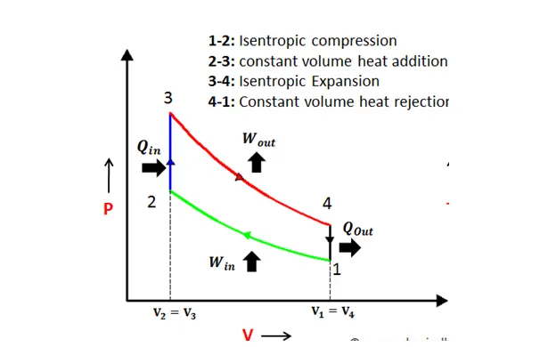
The 4 different points are shown in the pic with the properties.
Mathematical Equations-
The Otto cycle is a little heavy on the side of the equation but the processes are simples.
calculating swept volume and clearance volume
v_swept=(pi/4)*bore^2*stroke;
v_clearance=v_swept/(cr-1);
v1=v_swept+v_clearance;
where ,
v_swept= swept volume
v_clearance= clearance volume
v1= volume at point 1
Process 1-
1-2: Isentropic compression
In this piston compresses the fuel in the engine and the equation for the variable are-
v1=v_swept+v_clearance;
Process 2-
2-3: constant heat addition
p2v2^gamma=p1v1^gamma| p2=p1*v1^gamma/v2 |cr=v1/v2
p2=p1*cr^gamma;
t2=p2*v2*t1/(p1*v1);
Process 3-
3-4- isentropic expansion
v3=v2;
p3v3/t3=p2v2/t2 | p3=p2*v2*t3/v3
p3=p2*t3/t2;
Process 4-
4-1- the constant volume of heat rejection
v4=v1;
p3v3^gamma=p4v4^gamma | p4=p3*cr^gamma
p4=p3*(v3/v4)^gamma;
where,
cr= compression ratio
p1= pressure at point 1
p2= pressure at point 2
p3= pressure at point 3
p4= pressure at point 4
v1= volume at point 1
v2= volume at point 2
v3= volume at point 3
v4= volume at point 4
t1= temp. at point 1
t2 = temp. at point 2
t3= temp. at point 3
t4= temp. at point 4
For plotting the curve-
For process 1 compression-
constant_c=p1*v1^gamma;
v_compression=engine_kinematics(0.1,0.1,0.15,12,180,0);
p_compression=constant_c./v_compression.^gamma;
For process 3 expansion-
constant_c=p3*v3^gamma;
v_expansion=engine_kinematics(0.1,0.1,0.15,12,0,180);
p_expansion=constant_c./v_expansion.^gamma;
where ,
v_compression= compression volume
p_compression= compression pressure
v_expansion= expansion volume
p_expansion= expansion pressure
calculating thermal efficiency
thermal_efficiency= 1-(1/cr^(gamma-1))
efficiency_percent=thermal_efficiency*100
Matlab Code-
Plotting the points for the Otto cycle-
clear all
close all
clc
%inputs
gamma=1.4;
t3=2300;
%state variable at 1
p1=101325;
t1=500;
%engine geometry
bore=0.1;
stroke=0.1;
con_rod=0.15;
cr=12;
%calculating the swept vol and clearance vol
v_swept=(pi/4)*bore^2*stroke;
v_clearance=v_swept/(cr-1);
v1=v_swept+v_clearance;
v2=v_clearance;
%state variable at 2
%p2v2^gamma=p1v1^gamma
%p2=p1*(cr)^gamma
p2=p1*(cr)^gamma;
%p1v1/t1=p2v2/t2 | t2=p2*v2*t1/(p1*v1)
t2=p2*v2*t1/(p1*v1);
%state variable at point 3
v3=v2;
%p3v3/t3=p2v2/t2 |p3=p2*t3/t2
p3=p2*t3/t2;
%sate variable at 4
v4=v1;
%p3v3^gamma=p4v4^gamma |p4=p3*(v3/v4)^gamma
p4=p3*(v3/v4)^gamma;
figure(1)
hold on
plot(v1,p1,'*','color','r')
plot(v2,p2,'*','color','r')
plot(v3,p3,'*','color','r')
plot(v4,p4,'*','color','r')
grid on
Outputs/Results-
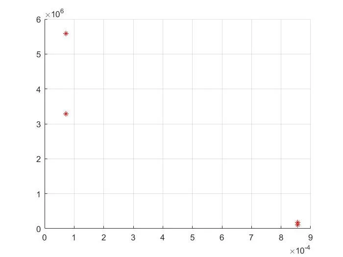
Explanation-
The code has successfully plotted the points on the graph
Plotting the curve-
clear all
close all
clc
%inputs
gamma=1.4;
t3=2300;
%state variable at 1
p1=101325;
t1=500;
%engine geometry
bore=0.1;
stroke=0.1;
con_rod=0.15;
cr=12;
%calculating the swept vol and clearance vol
v_swept=(pi/4)*bore^2*stroke;
v_clearance=v_swept/(cr-1);
v1=v_swept+v_clearance;
v2=v_clearance;
%state variable at 2
%p2v2^gamma=p1v1^gamma
%p2=p1*(cr)^gamma
p2=p1*(cr)^gamma;
%p1v1/t1=p2v2/t2 | t2=p2*v2*t1/(p1*v1)
t2=p2*v2*t1/(p1*v1);
%state variable at point 3
v3=v2;
%p3v3/t3=p2v2/t2 |p3=p2*t3/t2
p3=p2*t3/t2;
%sate variable at 4
v4=v1;
%p3v3^gamma=p4v4^gamma |p4=p3*(v3/v4)^gamma
p4=p3*(v3/v4)^gamma;
figure(1)
hold on
plot(v1,p1,'*','color','r')
plot(v2,p2,'*','color','r')
plot(v3,p3,'*','color','r')
plot(v4,p4,'*','color','r')
plot([v1 v2 v3 v4],[p1 p2 p3 p4],'linewidth',2)
grid on
Outputs/Results-
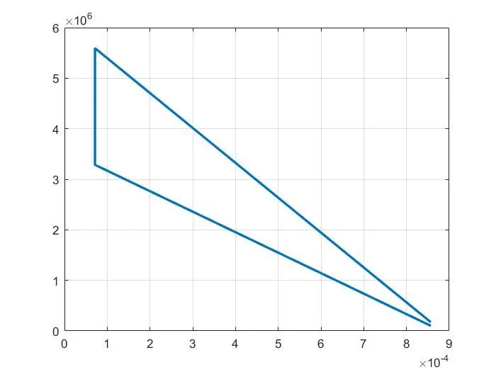
Explanation-
The line joining the point isn’t the real process. The graph here plotted to have the straight line whereas the real process have the curve
Function-
The function is a mathematical variable whose are dependent on the other given inputs. These are very useful in engineering as they come in handy in solving some complex mathematical system.
We will be using the function command of Matlab for plotting the exact curve for the Otto cycle.
Matlab Code for function-
function [V]=engine_kinematics(bore,stroke,cond_rod,cr,start_crank,end_crank)
a=stroke/2;
R=cond_rod/a;
v_s=pi/4*bore^2*stroke;
v_c=v_s/(cr-1);
theta=linspace(start_crank,end_crank,100);
term1=0.5*(cr-1);
term2=R+1-cosd(theta);
term3=(R^2-sind(theta).^2).^0.5;
V=(1+term1*(term2-term3)).*v_c;
end
For expansion plotting-
Inputs-
v=engine_kinematics(0.1,0.1,0.15,12,0,180)
Outputs/Results-
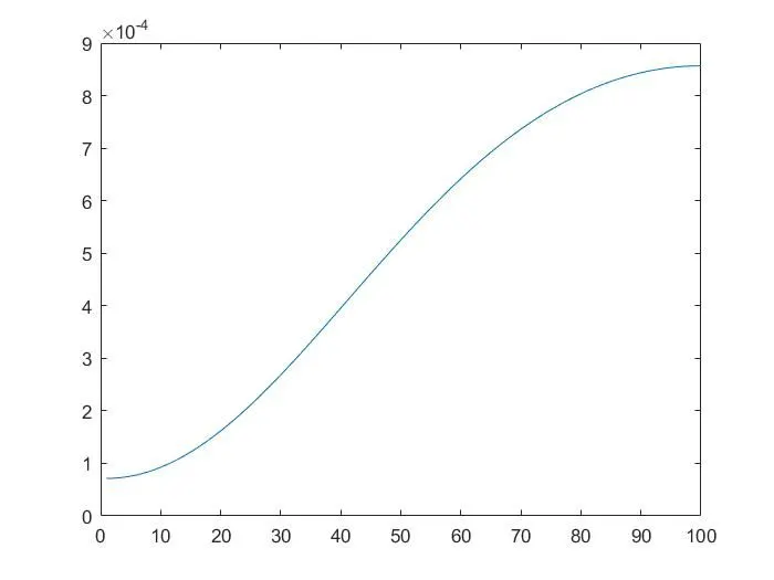
Explanation-
The graph for the volume expansion is plotted for the cycle.
For compression plotting-
Inputs
v=engine_kinematics(0.1,0.1,0.15,12,180,0)
Outputs/Results-
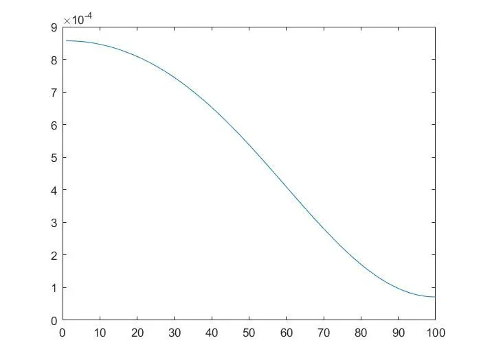
Explanation-
The graph for the volume compression for the angle 180 to 0 is being plotted with the curve this curve is very useful as it helps us know the exact volume compression in the process which can be plotted with the point for creating the graph.
For Otto cycle-
Inputs
v=engine_kinematics(0.1,0.1,0.15,12,0,720)
Outputs/Results-
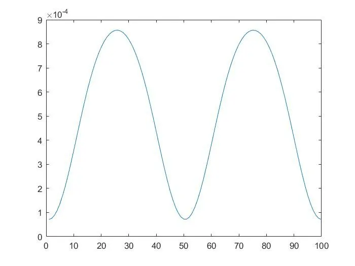
Explanation-
The volume cycle for 1 cycle has to be plotted from 0 to 720 degree.
Final iteration-
In this, we will plot the cycle for the Otto cycle.
Final code-
clear all
close all
clc
%inputs
gamma=1.4;
t3=2300;
%at state variable
p1=101325;
t1=5000;
%engine geometric parameter
bore=0.1;
stroke=0.1;
cond_rod=0.15;
cr=12;
%calculating swept volume and clearance volume
v_swept=(pi/4)*bore^2*stroke;
v_clearance=v_swept/(cr-1);
v1=v_swept+v_clearance;
constant_c=p1*v1^gamma;
v_compression=engine_kinematics(0.1,0.1,0.15,12,180,0);
p_compression=constant_c./v_compression.^gamma;
%at state 2
v2=v_clearance;
%p2v2^gamma=p1v1^gamma| p2=p1*v1^gamma/v2 |cr=v1/v2
%p2=p1*v1^gamma/v2 | p2=p1*cr^gamma
p2=p1*cr^gamma;
%p1v1/t1=p2v2/t2 | t2=p2*v2*t1/p1*v1
t2=p2*v2*t1/(p1*v1);
%at state point 3
v3=v2;
%p3v3/t3=p2v2/t2 | p3=p2*v2*t3/v3
p3=p2*t3/t2;
constant_c=p3*v3^gamma;
v_expansion=engine_kinematics(0.1,0.1,0.15,12,0,180);
p_expansion=constant_c./v_expansion.^gamma;
% at state point 4
v4=v1;
%p3v3^gamma=p4v4^gamma | p4=p3*cr^gamma
p4=p3*(v3/v4)^gamma;
%plotting
hold on
plot(v1,p1,'*','color','r')
plot(v_compression,p_compression,'linewidth',1)
plot(v2,p2,'*','color','r')
line([v2 v3],[p2 p3],'linewidth',1)
plot(v3,p3,'*','color','r')
plot(v_expansion,p_expansion,'linewidth',1)
plot(v4,p4,'*','color','r')
line([v4 v1],[p4 p1],'linewidth',1)
xlabel('volume')
ylabel('pressure')
%calculating thermal efficiency
thermal_efficiency= 1-(1/cr^(gamma-1));
efficiency_percent=thermal_efficiency*100;
Outputs/Results-
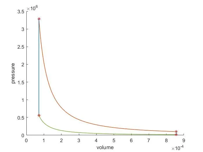
efficiency_percent =
62.9893
Explanation-
The final graph is being plotted and we can know the volume change and the pressure during the different stages of the cycle.
As well the thermal efficiency has been calculated and it is 62.98%.
Errors-
1.
The formula for p_compression=constant_c./v_compression^gamma but I forgot to raise the power of gamma.

2.
The formula for p_expansion=constant_c./v_expansion^gamma but I forgot to raise the power of gamma and forgot to change p3*v3.

3.
This is the mathematical error that I did. This formula should be-
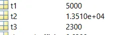
t2=p2*v2*t1/(p1*v1)
I didn’t put the bracket and the value of t2 have changed.
The value of t2 came out.
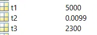
Whereas the value was
4.
Replaced v3/v4 as cr
Whereas v3/v4 is not equal to the compression ratio.

Conclusion-
The Plot for P vs V have been plotted correctly
The thermal efficiency is 62.98%