2r Robotics arm Simulation
AIM-
The Simulation of Forward Kinematics of a 2R Robotic Arm
Objective-
1 to plot the work area for the Robotic Arm
2 To simulate the Arm using MATLAB
Introduction-
The robotic arm is the Mechanical system. The robot arm is capable of doing simple as well as difficult job in the manufacturing facility.
As the Automation is increasing owing with the efficiency and the time for production is going we need these type of simple arms for the many things.
These type of arms can be used for jobs like picking and placing things, welding and so on…
Theory-
The robotic arm is the Mechanical system with the integration of the electronic it becomes very useful for efficiency.
The Robotic arm consists of 2 or more arms with multiple joint for its movement in the rotational and translation motion. The joint has a motor that helps the arm in motion and the end-effector is the point that is used for doing the job.
Calculations
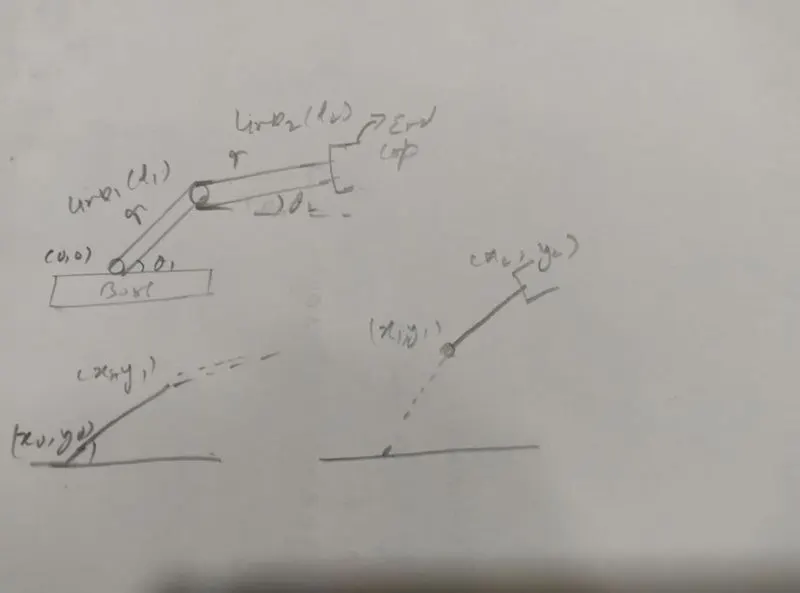
Inputs
L1=link1=1
L2=link2=0.5
Ɵ1= angle between the base and the link1
Ɵ2=angle between the link2 and the axis
We will be calculating the coordinates first
X0=0
Y0=0
X1=l1*cosƟ1
Y2=l2*sinƟ1
X2=x1+l2*cosƟ2
Y2=y1+l2*cosƟ2
Codes-
We will code with the itineraries
Code 1 – for single line plot
%kinematics of the robotic arm
clear all
close all
clc
%inputs
l1=1;
l2=0.5;
theta1=30;
theta2=45;
%coordinate
x0=0;
y0=0;
x1=l1*cosd(theta1);
y1=l1*sind(theta1);
x2=x1+l2*cosd(theta2);
y2=y1+l2*sind(theta2);
%ploting
line([x0 x1],[y0 y1],'linewidth',2,'color','r')
line([x1 x2],[y1 y2],'linewidth',2,'color','b')
Result/plot-
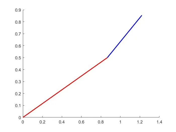
Explanation-
The plot shows the 2 arms of the robot at a particular angle the endpoint of the link2 is where the end effector is attached and it will hold the things or hold the welding rod
Conclusion-
From this single angle, the graph can be plotted and we can change the angle manually but this isn’t a better way to calculate the area under the arm.
So, we will change the code a little for better understanding.
Code 2- with for loop
%kinematics of the robotic arm
clear all
close all
clc
%inputs
l1=1;
l2=0.5;
theta1=linspace(0,90,10);
theta2=linspace(0,90,10);
%coordinate
x0=0;
y0=0;
for i=1:length(theta1)
THETA1=theta1(i);
for j=1:length(theta2)
THETA2=theta2(j);
x1=l1*cosd(THETA1);
y1=l1*sind(THETA1);
x2=x1+l2*cosd(THETA2);
y2=y1+l2*sind(THETA2);
%ploting
line([x0 x1],[y0 y1],'linewidth',2,'color','r')
line([x1 x2],[y1 y2],'linewidth',2,'color','b')
end
end
Result/plot-
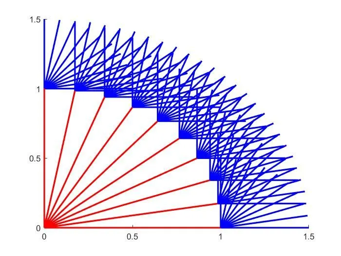
Explanation-
The plot shows the 2 arms of the robot at various angle theta1 as well as theta2. The plotted graph can help us in knowing the area under the arm.
Conclusion-
From the various angle using the linspace and the for loop command, the graph can be plotted but this isn’t a better way to calculate the area under the arm.
So, we will change the code a little for better understanding.
Code 3- multiple charts
%kinematics of the robotic arm
clear all
close all
clc
%inputs
l1=1;
l2=0.5;
theta1=linspace(0,90,5);
theta2=linspace(0,90,5);
%coordinate
x0=0;
y0=0;
ct=1
for i=1:length(theta1)
THETA1=theta1(i);
for j=1:length(theta2)
THETA2=theta2(j);
x1=l1*cosd(THETA1);
y1=l1*sind(THETA1);
0
x2=x1+l2*cosd(THETA2);
y2=y1+l2*sind(THETA2);
%ploting
figure(ct)
line([x0 x1],[y0 y1],'linewidth',2,'color','r')
line([x1 x2],[y1 y2],'linewidth',2,'color','b')
ct=ct+1
end
end
Result/plot-
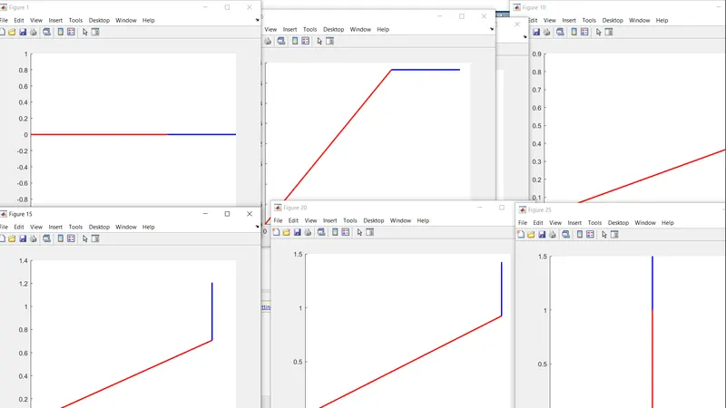
Explanation-
The plot shows the 2 arms of the robot at various angle theta1 as well as theta2. The plotted graph are in 25 different figure we can notice the area.
Conclusion-
From the various angle using the linspace and the for loop command, the graph can be plotted but this isn’t a better way to calculate the area under the arm.
So, we will change the code a little for a better understanding
Code 4- video
clear all
close all
clc
%inputs
l1=1;
l2=0.5;
theta1=linspace(0,90,20);
theta2=linspace(0,90,20);
ct=1;
for i=1:length(theta1)
THETA1=theta1(i);
for j=1:length(theta2)
THETA2=theta2(j);
x0=0;
y0=0;
x1=l1*cosd(THETA1);
y1=l1*sind(THETA1);
x2=x1+l2*cosd(THETA2);
y2=y1+l2*sind(THETA2);
%ploting
plot([x0 x1],[y0 y1],[x1 x2],[y1 y2],'linewidth',2)
axis([-0.1 1.5 0 1.5])
pause(0.3)
M(ct)=getframe(gcf);
ct=ct+1;
end
end
movie(M)
videofile=VideoWriter('forward_kinematic.avi','Uncompressed AVI')
open(videofile);
writeVideo(videofile,M);
close(videofile)
Result/plot-
Video link-
YouTube- https://youtu.be/TTIfXZJN_3Y
drive- https://drive.google.com/file/d/1Fb-_GhVZwWkku2zWCfiF9q10VTTtHR4B/view?usp=sharing
Explanation -
The video shows us the exact simulation of the robotic arm and while noticing the end effector at the end of the link you we can get the area under the scope or the working area of the robotic arm
Conclusion-
This is the final iteration in the code and we get the code that can get the frame of the robotic arm which can we see uploaded on YouTube as well as Drive.
End Conclusion-
The simulation of the two arms robotic shows the area it will cover under it or the working area.