Optimization Of Stalagmite Function Using Genetic Algorithm

MATLAB CODE(function file)

function[f]= stalagmite(input_vector)
    x= input_vector(1);
    y= input_vector(2);
    
    f_1_x= (sin(5.1*pi*x + 0.5))^6;
    f_1_y= (sin(5.1*pi*y + 0.5))^6;
    f_2_x= exp(-4*log(2)*(((x-0.0667)^2)/0.64));
    f_2_y= exp(-4*log(2)*(((y-0.0667)^2)/0.64));
    
    f= -1* f_1_x * f_2_x * f_1_y * f_2_y;
    
    %multiplication with -1 will generate maxima
    
end

MATLAB CODE(main file)

%program to find the global maxima of a stalagmite function
%using genetic algorithm 

%creating vectors in the known bounds
x= linspace(0,0.6,150);
y=linspace(0,0.6,150);
iterations= 100;
%creating 2D arrays out of the vectors
[xx yy]= meshgrid(x,y);


%evaluating the stalagmite function
for i= 1:length(xx)
    for j= 1:length(yy)
        input_vector(1)= xx(i,j);
        input_vector(2)= yy(i,j);
        f(i,j)= stalagmite(input_vector);
    end
end


%study 1
%unbounded
tic %to start the time measurement
for i=1:iterations
[inputs,fun_value(i)]= ga(@stalagmite,2);
x_output(i)= inputs(1);
y_output(i)= inputs(2);
end

time_elapsed_1=toc

figure(1)
subplot(2,1,1)
hold on
colorbar
surfc(xx,yy,f)
shading interp
plot3(x_output,y_output,fun_value,'marker','o','markerSize',3)
xlabel('x value')
ylabel('y value')
title('unbounded study')
subplot(2,1,2)
plot(fun_value)
xlabel('no. of iterations')
ylabel('maximum value')

%study 2
%with upper and lower bounds
tic
for j= 1:iterations
  [inputs fun_value(j)]= ga(@stalagmite, 2,[],[],[],[],[0;0],[1;1]);
  x_output(j)= inputs(1);
y_output(j)= inputs(2);
end

time_elapsed_2=toc

figure(2)
subplot(2,1,1)
colorbar
hold on
surfc(xx,yy,f)
shading interp
plot3(x_output,y_output,fun_value,'marker','o','markerSize',3)
xlabel('x value')
ylabel('y value')
title('bounded study')
subplot(2,1,2)
plot(fun_value)
xlabel('no. of iterations')
ylabel('maximum value')

%study 3
%increasing iterations by increasing the population size

options= optimoptions('ga','populationSize',200);
tic
iterations= 100;
for k= 1:iterations
  [inputs fun_value(k)]= ga(@stalagmite,2,[],[],[],[],[0;0],[1;1],[],[],options);
  x_output(k)= inputs(1);
  y_output(k)= inputs(2);
  
end

time_elapsed_3= toc

  figure(3)
subplot(2,1,1)
colorbar
hold on
surfc(xx,yy,f)
shading interp
plot3(x_output,y_output,fun_value,'marker','o','markerSize',3)
xlabel('x value')
ylabel('y value')
title('bounded study with modified population size')
subplot(2,1,2)
plot(fun_value)
xlabel('no. of iterations')
ylabel('maximum value')

AIM : Optimization of a stalagmite function using Genetic Algorithm.

The following objectives are achieved through this project :

· Performing optimization of the function using MATLAB.

· Finding the global maxima of the same function.

BACKGROUND : Genetic Algorithm is an optimization technique through a iterative procedure. The procedure followed is analogous to the one used by Charles Darwin in his theory of natural selection.

The algorithm follows a binary method but unlike other conventional optimization techniques which focus on improving a single solution, GA works on the improvement on a set of solution also called as population.

The GA produces successive hypotheses or population using 3 combination techniques, namely,

Mutation- applying random changes to individual parents to form children.

Crossover- combining two parents to form children for the next generation.

Selection- select the individuals called ‘parents’ that contribute to the population of the next generation.

As a result the offspring generation produced every time is a better version or improved version of its parent generation. Apart from having plenty of advantages, the GA possesses a disadvantage as well. The GA has to be designed very carefully as one unfavorable choice of operators may bring up entirely different results. Hence, a proper knowledge of basics and the context is an important prerequisite while solving any problem using Genetic Algorithm.

In our context, Genetic Algorithm can be used to solve both linear and non-linear optimization problems based on natural selection. Over successive generations, the population ultimately evolves towards on ‘optimal solution’. The GA can be applied to a variety of optimization problems which are not suitable for conventional methods including problems with discontinuous functions, non-differentiable functions or highly non-linear functions.

In our problem the following stalagmite has to be optimized to obtain a global maxima.

f(x,y)= f_1,x * f_2,x * f_1,y * f_2,y

f_1,x = [sin(5.1*pi*x + 0.5)]⁶

f_1,y= [sin(5.1*pi*x + 0.5)]⁶

f_2,x= exp[-4*ln2*(x-0.0667)²/0.64]

f_2,y= exp[-4*ln2*(y-0.0667)²/0.64]

Genetic Algorithm has the following syntax :

x= ga(fun,nvars)

x= ga(fun,nvars,A,b)

x= ga(fun,nvars,A,b,Aeq,beq)

x= ga(fun,nvars,A,b,Aeq,beq,lb,ub)

x= ga(fun,nvars,A,b,Aeq,beq,lb,ub,nonlcon)

x= ga(fun,nvars,A,b,Aeq,beq,lb,ub,nonclon,options)

x= ga(fun,nvars,A,b,[],[],lb,ub,nonclon,IntCon)

x= ga(fun,nvars,A,b,[],[],lb,ub,nonclon,IntCon,options)

x= ga(problem)

[x,fval]= ga(__)

[x,fval,exitflag,output]= ga(__)

[x,fval,exitflag,output,population,scores]= ga(__)

SOLUTION ALGORITHM

1. The program begins with the clear all, close all and clc commands to free up the command window and the workspace.

2. We will create two input vectors using linspace commands followed by generation of 2D arrays of the two vectors. These 2 vectors will basically act as inputs for the calculation of our stalagmite function.

3. The optimization function will be calculated in a separate script file and will be called in the main file.

4. Three separate studies will be performed using genetic algorithm and the time elapsed to perform each study will be recorded as well.

5. The working of GA is summarized in the following steps :

· The solution begins with the evaluation of an initial population.

· Then out of the initial population, it will select a few good solutions for reproduction.

· Then we will generate new population through selection, mutation and crossover followed by evaluation of new population.

· This process of generating new generations will be continued until the algorithm coverges.

· The convergence can take place through many criteria such as fixed number of generations, when the best fitness function value is no longer changing or changing by a very small amount.

6. The code for the entire program will be written in MATLAB.

OUTPUT

The following output is obtained after running the code :

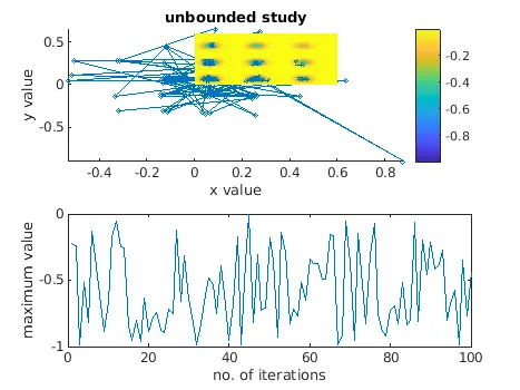
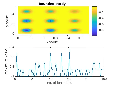
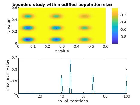
· The time elapsed for the unbounded study is 12.3583 seconds.

· The time elapsed for the bounded study is 11.7885 seconds.

· The time elapsed for the study with increased iterations is 34.1851 seconds.

ERROR

Some errors in the form of typing mistakes occurred and were rectified.

REFERENCES

· https://www.sciencedirect.com/topics/engineering/genetic-algorithm

· https://www.mathworks.com/help/gads/what-is-the-genetic-algorithm.html

· https://www.mathworks.com/help/gads/examples/genetic-algorithm-options.html?s_tid=mwa_osa_a

· https://www.mathworks.com/help/gads/ga.html

$f(x,y)=f_{1,x}*f_{2,x}*f_{1,y}*f_{2,y}$

dc