Optimization of stalagmite function using Genetic Algorithm
AIM
To find the global maxima of the stalagmite function using Genetic Algorithm in MATLAB.
OBJECTIVES
- Code the stalagmite function in MATLAB
- Optimize stalagmite function and find the global maxima of the function.
- Study 3 case of options of Genetic Algorithm 'ga' in MATLAB.
BASIC STUDY
Genetic algorithm solves smooth or non smooth optimization problems with any types of constraints, including integer constraints. It is a stochastic, population-based algorithm that searches randomly by mutation and crossover among population members.
Solver 'ga' finds minimum of function using genetic algorithm.
How the genetic algorithm works:
The algorithm begins by creating a random initial population.
The algorithm then creates a sequence of new populations.
At each step, the algorithm uses the individuals in the current generation to create the next population.
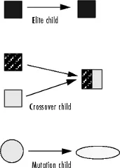
- Selects members, called parents, based on their expectation.
- Some of the individuals in the current population that have lower fitness are chosen as elite. These elite individuals are passed to the next population.
- Produces children from the parents. Children are produced either by making random changes to a single parent—mutation—or by combining the vector entries of a pair of parents—crossover.
- Replaces the current population with the children to form the next generation.
The algorithm stops when one of the stopping criteria is met.
EQUATIONS
The stalagmite function
INITIAL AND BOUNDARY CONDITIONS
Case 1
-
-
-
-
-
-
-
-
-
-
-
- No bound values
- Default (50) population
-
-
-
-
-
-
-
-
-
-
Case 2:
X bound values
Xmin :0
Xmax :0.6
Y bound values
Xmin :0
Ymax :0.6
Default (50) population
Case 3:
X bound values
Xmin :0
Xmax :0.6
Y bound values
Xmin :0
Ymax :0.6
Initial population 250
MATLAB PROGRAM
The stalagmite function
% The stalagmite function
function [stalagmite] = stalagmiteFunction(input_vector)
    x = input_vector(1);
    y = input_vector(2);
    f1x = (sin((5.1*pi*x)+0.5))^6; % term 1
    f1y = (sin((5.1*pi*y)+0.5))^6; % term 2
    f2x = exp((-4*log(2)*(x-0.0667)^2)/0.64); % term 3
    f2y = exp((-4*log(2)*(y-0.0667)^2)/0.64); % term 4

    stalagmite = -(f1x*f1y*f2x*f2y);
end
Case 1: Unbound Inputs and default (50) population
% Program to find global maxima using genetic algorithm
close all
clear all
clc
% Field of interest of optimisation
x = linspace(0,0.6,150);
y = linspace(0,0.6,150);
num_cases =50;
[xx yy] = meshgrid(x,y);
% Creating Data points of stalagmite Function
for i = 1:length(xx)
    for j = 1:length(yy)
        input_vector(1) = xx(i,j);
        input_vector(2) = yy(i,j);
        f(i,j) = stalagmiteFunction(input_vector);
    end
end
% Iterations of genetic algorithm
tic
for i = 1:num_cases
    [inputs, fopt(i)] = ga(@stalagmiteFunction,2);
    xopt(i) = inputs(1);
    yopt(i) = inputs(2);
end
toc
% Ploting results
figure(1)
suptitle('Genetic Algorithm Unbound Inputs')
subplot(2,1,1)
hold on
surfc(xx,yy,-f)
shading interp
title('Genetic Algorithm Unbound Inputs')
plot3(xopt,yopt,-fopt,'marker','o','markersize',5)
xlabel('x axis')
ylabel('y axis')
zlabel('f(x,y)')
subplot(2,1,2)
plot(-fopt)
xlabel('Iterations')
ylabel('Global Maxima')
title('Global Maxima vs Iterations')
axis([0 50 0 1.5])
Case 2: Bound Inputs and default (50) population
% Program to find global maxima using genetic algorithm
close all
clear all
clc
% Field of interest of optimisation
x = linspace(0,0.6,150);
y = linspace(0,0.6,150);
num_cases =50;
[xx yy] = meshgrid(x,y);
% Creating Data points of stalagmite Function
for i = 1:length(xx)
    for j = 1:length(yy)
        input_vector(1) = xx(i,j);
        input_vector(2) = yy(i,j);
        f(i,j) = stalagmiteFunction(input_vector);
    end
end


% Defining Population size
options = optimoptions('ga');
options = optimoptions(options, 'PopulationSize',250);

% Iterations of genetic algorithm Bound Inputs
tic
for i = 1:num_cases
    [inputs, fopt(i)] = ga(@stalagmiteFunction,2,[],[],[],[],[0;0],[0.6;0.6]); % Bound Inputs
    xopt(i) = inputs(1);
    yopt(i) = inputs(2);
end
toc
% Ploting results
figure(1)
suptitle('Genetic Algorithm Bound Inputs')
subplot(2,1,1)
hold on
surfc(xx,yy,-f)
shading interp
title('Genetic Algorithm Bound Inputs')
plot3(xopt,yopt,-fopt,'marker','o','markersize',5)
xlabel('x axis')
ylabel('y axis')
zlabel('f(x,y)')
subplot(2,1,2)
plot(-fopt)
xlabel('Iterations')
ylabel('Global Maxima')
title('Global Maxima vs Iterations')
axis([0 50 0 1.5])
Case 3: Bound Inputs and 250 population
% Program to find global maxima using genetic algorithm
close all
clear all
clc
% Field of interest of optimisation
x = linspace(0,0.6,150);
y = linspace(0,0.6,150);
num_cases =50;
[xx yy] = meshgrid(x,y);
% Creating Data points of stalagmite Function
for i = 1:length(xx)
    for j = 1:length(yy)
        input_vector(1) = xx(i,j);
        input_vector(2) = yy(i,j);
        f(i,j) = stalagmiteFunction(input_vector);
    end
end

% Defining Population size
options = optimoptions('ga');
options = optimoptions(options, 'PopulationSize',250);
% Iterations of genetic algorithm Bound Inputs with increased Population size
tic
for i = 1:num_cases
    [inputs, fopt(i)] = ga(@stalagmiteFunction,2,[],[],[],[],[0;0],[0.6;0.6],[],[],options);
    xopt(i) = inputs(1);
    yopt(i) = inputs(2);
end
toc
% Ploting results
figure(1)
suptitle('Genetic Algorithm Bound Inputs with increased Population size')
subplot(2,1,1)
hold on
surfc(xx,yy,-f)
shading interp
title('Genetic Algorithm Bound Inputs with increased')
plot3(xopt,yopt,-fopt,'marker','o','markersize',5)
xlabel('x axis')
ylabel('y axis')
zlabel('f(x,y)')
subplot(2,1,2)
plot(-fopt)
xlabel('Iterations')
ylabel('Global Maxima')
title('Global Maxima vs Iterations')
axis([0 50 0 1.5]
EXPLANATION
Step 1: write a program for the stalagmite function in MATLAB
Step 2: Optimize stalagmite function and find the global maxima of the function with Unbound Inputs and no options.
Step 2: Optimize stalagmite function and find the global maxima of the function with Bound Inputs and no options.
Step 2: Optimize stalagmite function and find the global maxima of the function with Bound Inputs and with increased initial population.
Step 2: Study 3 cases Genetic Algorithm 'ga' in MATLAB.
RESULTS
Case 1: Unbound Inputs and default (50) population Time taken is 12.637761 seconds.
Case 2: Bound Inputs and default (50) population Time taken is 15.954995 seconds.
Case 3: Bound Inputs and 250 population Time taken is 42.235879 seconds.
CONCLUSION
Stalagmite function is coded in MATLAB and global maxima of the function is found using Genetic Algorithm 'ga' in MATLAB.
There different cases of Genetic Algorithm options are tried and compared for accuracy and time taken.
ERRORS
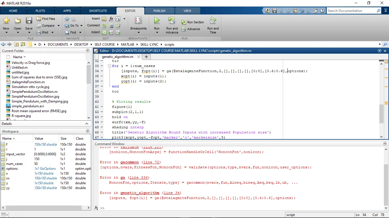
Correction
% Iterations of genetic algorithm Bound Inputs with increased Population size
tic
for i = 1:num_cases
    [inputs, fopt(i)] = ga(@stalagmiteFunction,2,[],[],[],[],[0;0],[0.6;0.6],[],[],options);
    xopt(i) = inputs(1);
    yopt(i) = inputs(2);
end
toc
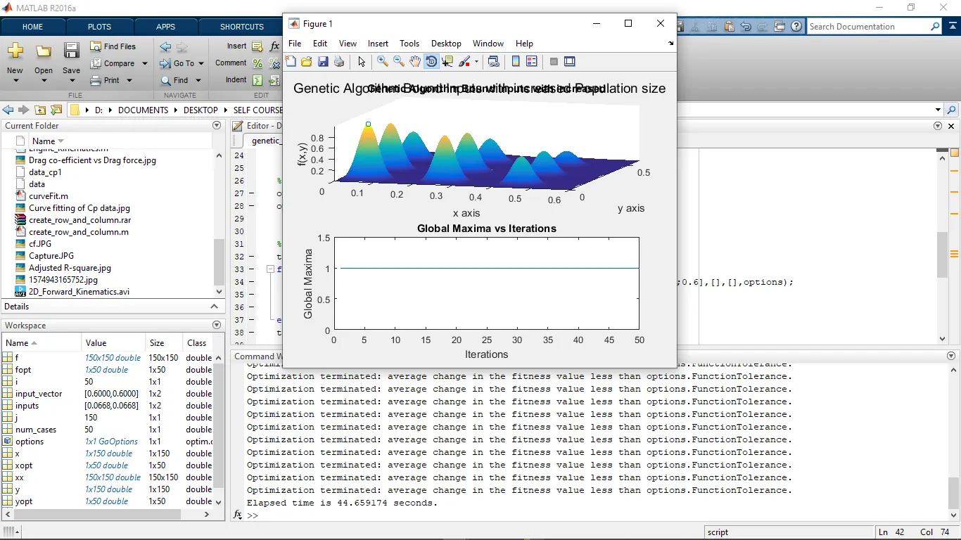
Correction
% Ploting results
figure(1)
suptitle('Genetic Algorithm Bound Inputs with increased Population size')
subplot(2,1,1)
hold on
surfc(xx,yy,-f)
shading interp
title('Genetic Algorithm Bound Inputs with increased')
plot3(xopt,yopt,-fopt,'marker','o','markersize',5)
xlabel('x axis')
ylabel('y axis')
zlabel('f(x,y)')
subplot(2,1,2)
plot(-fopt)
xlabel('Iterations')
ylabel('Global Maxima')
title('Global Maxima vs Iterations')
axis([0 50 0 1.5])
REFERENCES