Numerical and Experimental validation of PEM fuel cell.

Aim:

To find the optimal parameter of the fuel cell.

Objective:

• To improve the performance of PEM fuel cells with Serpentine flow channel and single flow channel by varying the working parameters.
• To achieve uniform reactants distribution with lower fuel consumption.

NOTE: Tool used to solve is COMSOL Multiphysics

Abstract:

A fuel cell is a device that has the potential to replace the Internal Combustion engine. It has the advantage of low emission or in such cases zero-emission. In this project, the Proton Exchange Membrane (PEM) fuel cell is taken for the study because of its desirable characteristics are Quick Startup over other fuel cells and low-Temperature Operation. In this project, a Single flow channel (A Micro Channel for Numerical Study) PEM Fuel cell is modeled and analyzed to obtain the optimum pressure from the range of 0.5 bar to 2 bar. Then it is applied to the serpentine flow model and then results are compared with the Experimental Setup.

Keywords: PEM Fuel cell, Single Flow channel, Serpentine Flow Channel

Introduction:

Fuel cell

• A fuel cell is a device that converts the chemical energy from a fuel into electricity through a chemical reaction with oxygen or another oxidizing agent.
• Their many types of fuel cell classified based on fuel usage they are given by

1. Proton Exchange Membrane (PEM) Fuel Cells
2. Direct Methanol Fuel Cells
3. Alkaline Fuel Cells
4. Phosphoric Acid Fuel Cells
5. Molten Carbonate Fuel Cells
6. Solid Oxide Fuel Cells
7. Regenerative Fuel Cell

• The most common fuel used in this process is hydrogen. Besides, hydrocarbons like natural gas and alcohols such as methanol were used.

PEM fuel cell:

Proton exchange membrane (PEM) fuel cells are also called polymer electrolyte membrane. PEM fuel cells can deliver high-power density and other advantages are low weight and volume, compared with other fuel cells. A solid polymer is used as an electrolyte in a PEM fuel cell and a platinum catalyst is present in the porous carbon electrodes. They require only hydrogen, oxygen from the air, and water to operate and they do not need corrosive fluids like other fuel cells. Hydrogen will be supplied to the fuel cell with the help of storage tanks. Proton exchange membrane fuel cells operate at relatively low temperatures. The low-temperature operation helps for a quick start (less warm-up time) and helps in reducing the wear on system components, which ends in better durability.

Transportation is the main application of PEM fuel cells and some other stationary applications. Due to their fast startup time, favorable power-to-weight ratio, and low sensitivity to orientation, PEM fuel cells are best suitable for use in passenger vehicles, such as cars and buses. These fuel cells have a wider impact on the environment because they control the emission of greenhouse gases. Fuel cells using hydrogen as fuel can work up to 40% efficiently. Hydrogen has low energy density, storing hydrogen is a difficult process. Some of the fuels having higher density are gasoline, LPG, ethanol, methanol, natural gas can be
used for fuel. However, the methanol needs to reform to hydrogen.

Methodology:

• Reason for Study
• Modeling the Single and Serpentine flow channels
• Numerical Study
• Post Process the results.

Reason for the Numerical study:

• Back Pressure (Reference pressure) influence the performance of the fuel cell most.
• The pressure is responsible for the uniform reactant distribution. To ensure the uniform reactants distribution over the channels.

Modeling for study:

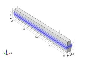
The Data for the modeling of the single and Serpentine flows were taken from the Literature Survey. The model is developed in the Solidworks with Dimension for the serpentine flow. The single flow channel is already loaded in the COMSOL Multiphysics so we can use the model for the project by changing the required parameter in the Pre-existing Method. For the case of the serpentine flow, we have to model the flow channel cross-section of 50x50mm and to import to the COMSOL Multiphysics and we can add require physical condition for the study.

For Single-flow:

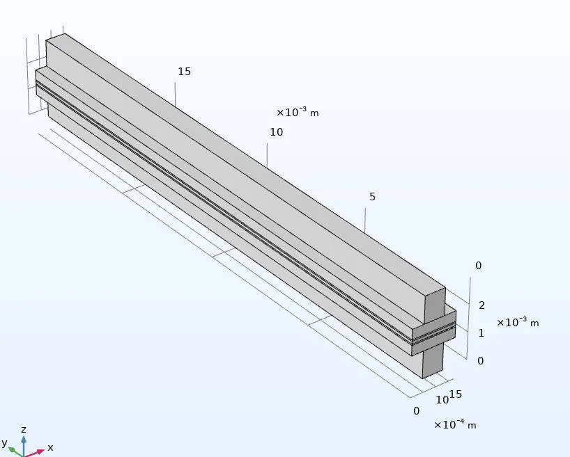
Design Parameters are given by

Following modeling parameters are taken for this project	Dimension and Values
•Length of the channel	: 0.02 [m]
•Channel Height	:1E-3 [m]
•Channel width	:1E-3[m]
•GDL width	: 380E-6[m]
•Porous electrode thickness	: 50e-6[m]
•Membrane thickness	: 100e-6[m]
Following are the conductivity of the model
•GDL	:222 [S/m]
•Membrane	: 9.825[S/m]
Following are the permeability of the model
•GDL	: 1.18e-11[m^2]
•Membrane	:3.622e-11[m^2]

For Serpentine Flow model:

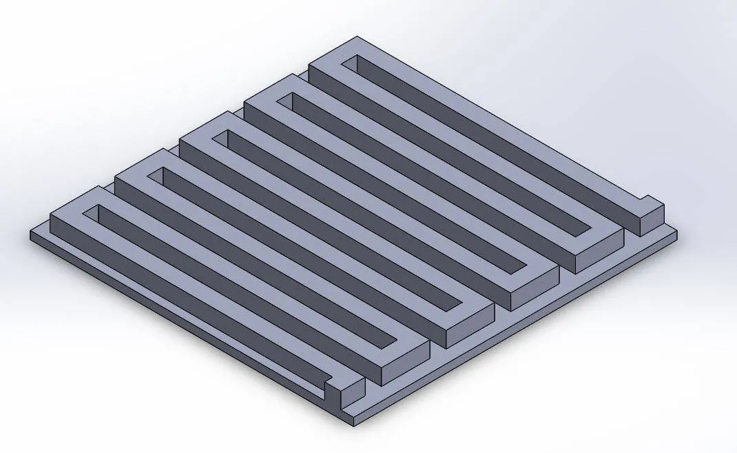
The serpentine flow is modeled in the Solidworks

The following parameters for modeling are

• Width of Rib: 2 mm
• Width of Channel: 2 mm
• Width of plate (B) : 50 mm
• Height of Channel: 2 mm
• Height of GDL: 0.3 mm
• Membrane thickness: 0.127 mm
• Catalyst layer: 0.08 mm

After the modeling, the model is imported into COMSOL Multiphysics.

Numerical study:

For single-flow:

The single flow model is imported into the workspace from the application library. The operation parameters are set into following

The voltage of Cell: 0.4 V – 0.9 V

The temperature of Cell: 313 K

The concentration of Oxygen: 40.88 mol/m^3

Cathode Inlet Hydrogen mass fraction: 0.023

Cathode Inlet Oxygen mass fraction: 0.228

The velocity of inlet: 2 m/s

The viscosity of fluid: 2.46×10^-5 Pa*s

The molar mass of Nitrogen: 0.028

The molar mass of water: 0.018

The molar mass of Oxygen: 0.032

Reference pressure : 0.5 -2.0×10^5 Pa

The physics for the study are imported to the model. The Navier-strokes equation provides the flow properties and Brinkmann's equation provides momentum transport by shear stress from the free channel and porous catalyst. The Brinkmann's Equation is an extension of the NS Equation given by

`rho(delu)/(delt)- grad.eta(gradu+(gradu)^T)-((eta/k)u+gradp-F)=0`

`grad.u=0`

Brinkmann's equation provides the Element properties in between the free channel and porous catalyst membrane. After Brinkmann's equation, the transport concentration species equation is added to the model for the numerical study. The Equation gives the transport of the ions in the fuel cell. In which the `j_i` is Flux- component. Omega (`Omega`) is the mass Diffusive flux. Where `R_i` is the reaction Co-efficient. The Transport concentration species equation gives

`grad.j_i+rho(u.grad)omega_i=R_i`

Finally, the secondary current equation is added to combine the transport species equation and Brinkmann Equation.

Initial Condition and Boundary Condition:

Step 1: The Material is added to the Imported model.

Step 2: The boundary condition like the inlet, outlet, GDL, Catalyst is selected.

Step 3:The study is run for the different back pressure ranges from the 0.5, 1, 1.5, and 2 bar. (Range is taken from the literature survey)

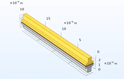
The above figure explains the Cathode Compartment of the single Flow channel. The Boundary Condition is given by the following

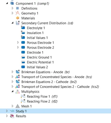
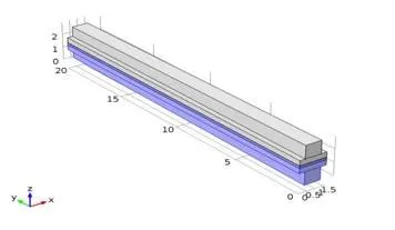
Membrane Element Assembly was given by

Reacting Flow in Porous Media (RFPM) given by

Meshing:

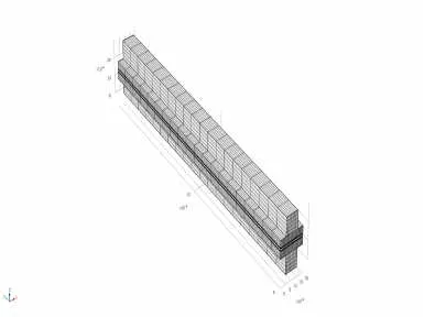
The meshing of the model is kept as the default. The mesh used in the model is TetraHexdral shape which provides the acceptable error within the stipulated time for the simulation time. The total cells in the Model are 51680.

Results and Discussion:

The Model is tested for the pressure range and voltage.

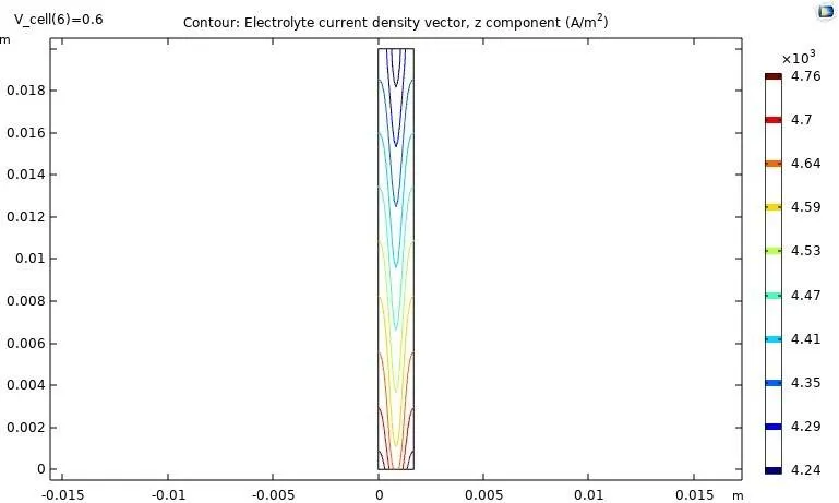
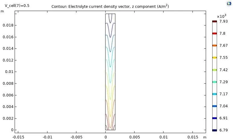
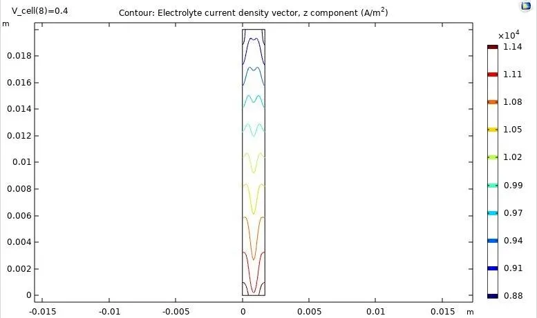
Single.1 to Single.4 shows the numerical analysis results of membrane current density in the single flow channel. Among these four different operating pressures and five different operating temperatures, PEM fuel cell with a single flow channel at 2.0 bar 40˚C gives the maximum current density of 1.17696`A/(cm^2)`

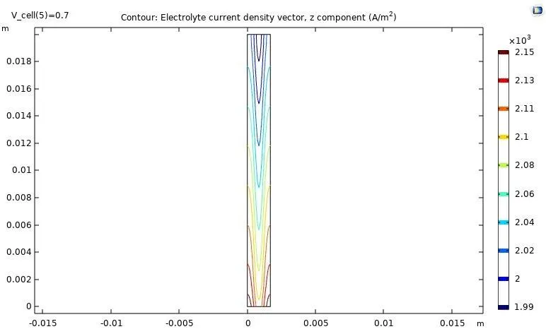
Single 1:Membrane current density at 0.5 bar and 60˚C [Single Flow Channel][Temperature is required for the Reactants flow]

Single 2:Membrane current density at 1 bar and 40˚C [Single Flow Channel]

Single 3:Membrane current density at 1.5 bar and 40˚C [Single Flow Channel]

Single 4:Membrane current density at 2 bar and 40˚C [Single Flow Channel]

Table: Current density at different pressure and temperature

[Single Flow Channel]

Sl.No.	Voltage (V) In Volts	Current Density (A) in `A/(cm^2)`
		0.5 bar & 60˚C	1.0 bar & 40˚C	1.5 bar & 40˚C	2.0 bar & 40˚C
1	0.40	0.67848	0.96021	1.0925	1.17696
2	0.45	0.59397	0.809891	0.91912	0.99186
3	0.50	0.49289	0.6606	0.75139	0.81394
4	0.55	0.38518	0.51672	0.59195	0.64527
5	0.60	0.27972	0.38226	0.44376	0.48856
6	0.65	0.18387	0.26154	0.31045	0.34708
7	0.70	0.10492	0.15982	0.19655	0.22498
8	0.75	0.04948	0.08306	0.10762	0.12758
9	0.80	0.019	0.03526	0.04859	0.06021
10	0.85	0.00629	0.01246	0.01802	0.02322
11	0.90	0.00194	0.00396	0.00586	0.00772

The tabulated numerical analysis results of a single flow channel for power density. Among these four different operating pressures and five different operating temperatures, a PEM fuel cell with a single flow channel at 2.0 bar 40˚C gives the maximum power density of 0.4707840 `W/(cm)^2`.

Sl.No.	Voltage (V) In Volts	Power density(`A/(cm^2)`)
		0.5 bar & 60˚C	1.0 bar & 40˚C	1.5 bar & 40˚C	2.0 bar & 40˚C
1	0.40	0.2713920	0.384084	0.4370000	0.4707840
2	0.45	0.2672865	0.364451	0.4136040	0.4463370
3	0.50	0.2464450	0.330300	0.3756950	0.4069700
4	0.55	0.2118490	0.284196	0.3255725	0.3548985
5	0.60	0.1678320	0.229356	0.2662560	0.2931360
6	0.65	0.1195155	0.170001	0.2017925	0.2256020
7	0.70	0.0734440	0.111874	0.1375850	0.1574860
8	0.75	0.0371100	0.062295	0.0807150	0.0956850
9	0.80	0.0152000	0.028208	0.0388720	0.0481680
10	0.85	0.0053465	0.010591	0.0153170	0.0197370
11	0.90	0.0017460	0.003564	0.0052740	0.0069480

Cathode oxygen concentration:

The numerical analysis results of Cathode oxygen concentration in the single flow channel. Among these four different operating pressures and five different operating temperatures, a PEM fuel cell with a single flow channel at 2.0 bar 40˚C gives the maximum Cathode oxygen concentration of 15.570 `(mol)/m^3`.

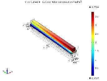
Figure 1: Cathode Oxygen Concentration at 0.5 bar and `60^0C` [Single Flow Channel]

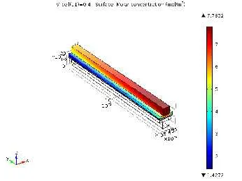
Figure 2: Cathode Oxygen Concentration at 1 bar and `40^0C` [Single Flow Channel]

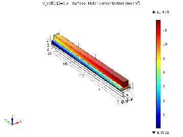
Figure 3:Cathode oxygen concentration at 1.5 bar & `40^0C`C [Single Flow Channel]

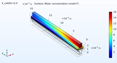
Figure 4:Cathode oxygen concentration at 2 bar & 40˚C [Single Flow Channel]

Anode Water Concentration:

The numerical analysis results of anode Hydrogen concentration in the single flow channel. Among these four different operating pressures and five different operating temperatures, a PEM fuel cell with a single flow channel at 2.0 bar `40^0`C gives the maximum Anode Hydrogen concentration of 73.972`(mol)/m^3`.

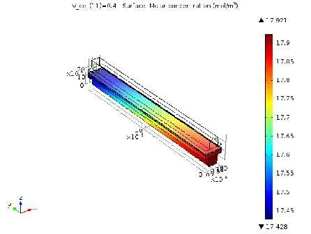
Fig 1: Anode Water Concentration at 0.5 bar & `60^0C`[Single Flow Channel]

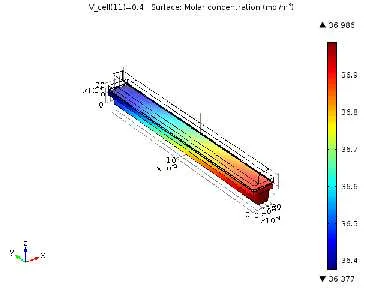
Fig 2: Anode Water Concentration at 1 bar & `40^0C`[Single Flow Channel]

Fig 3: Anode Water Concentration at 1.5 bar & `40^0C` [Single Flow Channel]

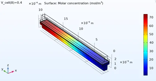
Fig 4: Anode Water Concentration at 2.0 bar & `40^0C`[Single Flow Channel]

Polarisation Curve:

The effect of change of temperature and pressure inside the cell for current and power densities of single flow channel PEM fuel cell. PEM fuel cells with a single flow channel at 2.0 bar `40^0C`C give the maximum current and power densities. (1.17696 `A/(cm^2)` & 0.470784 `W/(cm^2)` ).

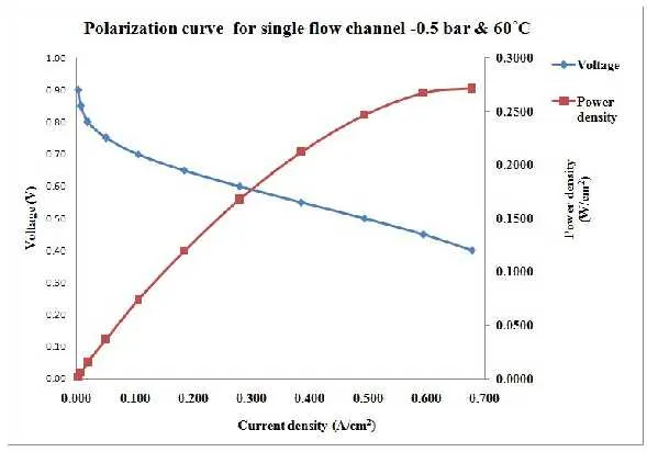
PolariZation Curve for the single Flow channel 0.5 bar and `60^0C`

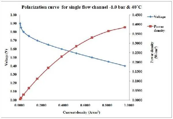
PolariZation Curve for the single Flow channel 1 bar and `40^0C`

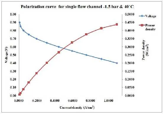
PolariZation Curve for the single Flow channel 1.5 bar and `40^0C`

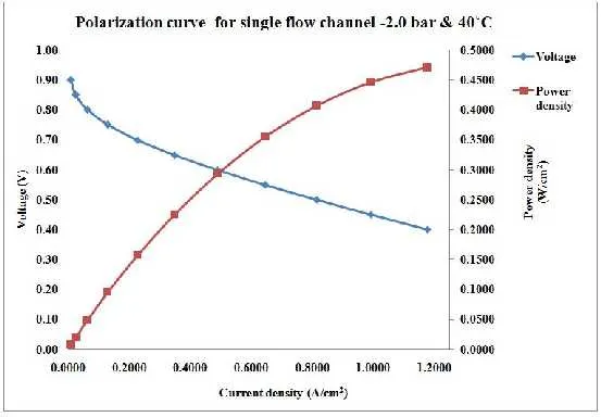
PolariZation Curve for the single Flow channel 2 bar and `40^0C`

From the numerical analysis, the following conclusions were made. Among the four different operating pressures and five different operating temperatures, the PEM fuel cell with a single flow channel at 2.0 bar and 40˚C gives a better performance than others.

SERPENTINE MODEL (50x50 mm):

For the Numerical study of the serpentine flow, the modeling was done in Solidworks and it was imported to the COMSOL Multiphysics software. There are certain steps to the Import the serpentine. Before the model is imported, we have to add the required physics for the simulation of the Fuel cell. The following are steps for the importing model. The New blank is selected and the 3D Model Option is selected. The following are the physics

• The major advantage of COMSOL Multiphysics is solving the two (or) More domains without the complex steps.
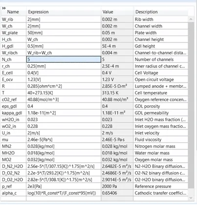
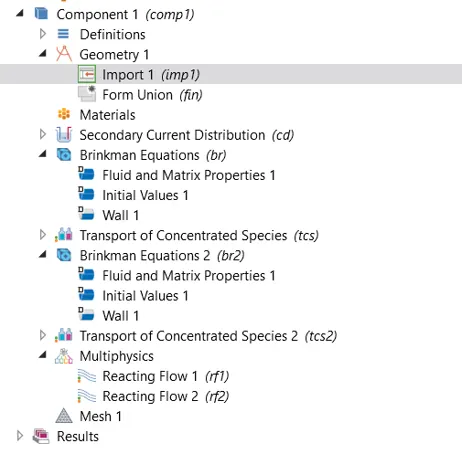
• For this project select the < Blank Model <3D < Batteries< add Secondary Current Distribution < add. The Transport Concentration species is added from the Reacting Porous media.
• The Reacting flow in porous media Provides the Brinkman equation and Transport Concentration Species in combination.

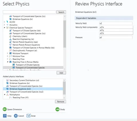
• After adding the physics, the Model is imported to the software.
• The Material and Operational Parameters are added to the imported Model.

Cell Voltage Lumped anode and membrane resistance	: 0.4V – 0.9V : 0.285 `(Ohm)/(cm)^2`
Cell temperature Oxygen reference concentration GDL permeability	: 323 K : 40.88 `(mol)/m^3` : 1.88×10-11 `m^2`
Cathode Inlet Hydrogen mass fraction	: 0.023
Cathode Inlet Oxygen mass fraction	: 0.228
Inlet velocity Fluid viscosity	: 2 m/s : 2.46×10-5 `Pa.s`
Nitrogen molar mass	: 0.028
Water molar mass	: 0.018
Oxygen molar mass Reference pressure	: 0.032 : `1X10^5 Pa`

• After that, the initial condition and Boundary condition is applied to the model. The Parameters are checked for the addition.

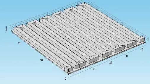
• The mesh model of PEMFC with serpentine 50×50 mm model is shown in the below figure.

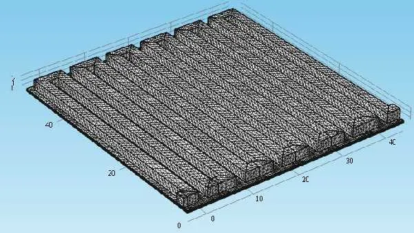
• The bottom channel and the GDL(Gas Diffusion Layer) area between the serpentine bend of the bottom channel have a finer mesh to resolve the channel-to-channel crossflow.
• The Total Number of Mesh elements in the Serpentine Flow is given by 245690 Cells.
• After the Meshing, the Study is added to the Model.

Result and Discussion:

The Membrane Current Density of the serpentine Flow is given by the

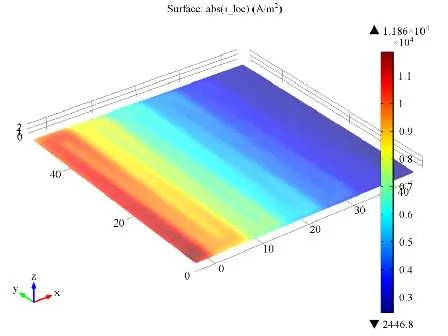
The numerical analysis results of membrane current density in serpentine 50×50mm model. It gives the maximum and minimum current density values at an operating voltage of 0.4 V is 1.186 `A/(cm^2)` and 0.24468`A/(cm^2)`.

The Tabulated numerical analysis results of current density in serpentine 50×50 mm model. Among these six different operating voltages, the PEM fuel cell with serpentine 50×50 mm model at 0.4 V gives the maximum current density of `A/(cm^2)`.

The current density of the serpentine 50×50 model

Sl.No.	Voltage (V) in Volts	Current density (A) in A/cm2
1	0.4	1.1860
2	0.5	0.9002
3	0.6	0.6049
4	0.7	0.3396
5	0.8	0.1289
6	0.9	0.0254

Power Density:

The tabulated numerical analysis results of power density in serpentine 50×50 mm model. Among these six different operating voltages, the PEM fuel cell with serpentine 50×50 mm model at 0.4V gives the maximum power density of 0.4744`W/(cm^2)`.

Power density values at different operating voltages

[Serpentine 50×50 mm model]

Sl.No.	Voltage (V) in Volts	Power density (P) in W/cm2
1	0.4	0.4744
2	0.5	0.4501
3	0.6	0.3629
4	0.7	0.2377
5	0.8	0.1031
6	0.9	0.0228

Cathode Oxygen Concentration:

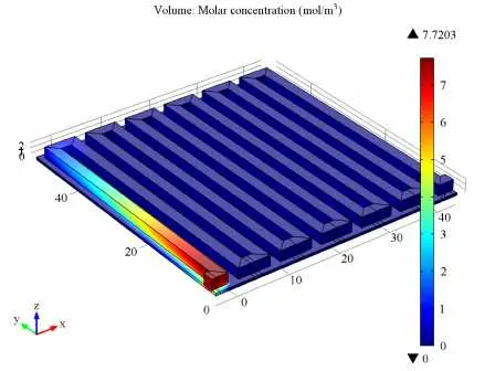
The numerical analysis results of cathode oxygen concentration in serpentine 50×50mm model. It gives the maximum and minimum value of cathode oxygen concentration at 0.4V operating voltage is 0 `(mol)/m^3` and 7.7203 `(mol)/m^3`.

GDL VELOCITY:

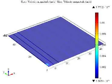
The numerical analysis results of GDL velocity in serpentine 50×50mm model. It gives the maximum and minimum value of GDL velocity at 0.4V operating voltage is 5.5039 x`10^-3m/s`and 5.7702 ×`10^-5 m/s` respectively.

GDL Pressure:

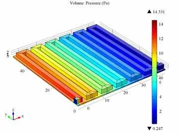
The numerical analysis results of GDL pressure in serpentine 50×50mm model. It gives the maximum and minimum value of GDL pressure at 0.4V operating voltage is 14.531 Pa and 0.247 Pa respectively.

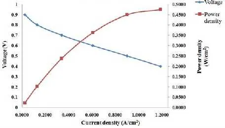
The polarization curve of the Serpentine Flow 50x50mm

Experimental Setup of Serpentine Flow:

The experimental setup of the PEM fuel cell is shown in the figure below. This is used to find out the current density and power density values of the PEM fuel cell with different flow channel designs. The flow channels are made of Graphite plate. The different flow paths on the graphite plate are machined by using CNC machines.

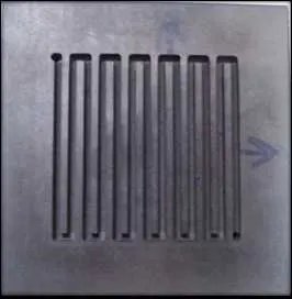
CNC Setup

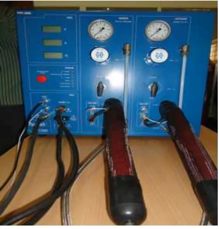
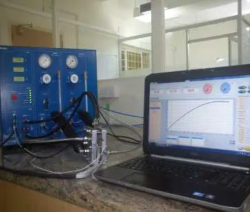
The Experimental setup with the data acquisition system is used to get the results for the PEM Fuel cell setup. The schematic diagram explains the Operations of the PEM Fuel cell.

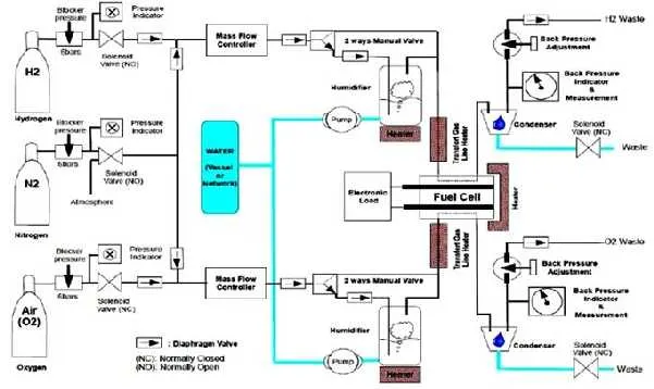
The experimental set up of PEM fuel cell arrangement with different controlling elements. Pure Hydrogen and oxygen are supplied to the fuel cell system using gas cylinders. Nitrogen is used as a purge gas for cleaning the fuel cell system.

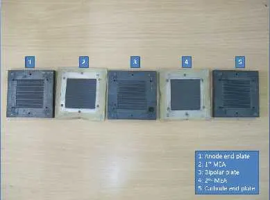
The above figure explains the Different parts of a real PEMFC.

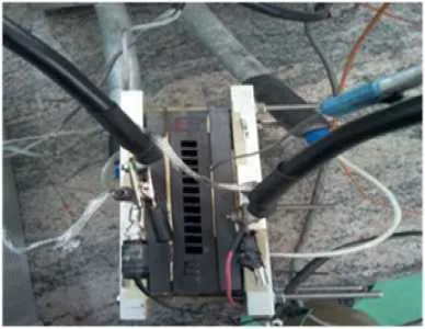
The figure explains PEM Fuel Setup. Once the study is done results are Compared with the Serpentine flow Numerical Model.

Results for the Experimental Setup

The Power and Current Densities of the PEM Fuel cell is given by

Voltage (V)	Current density (A) (`A/(cm^2)`)	Power density (P) (`W/(cm^2)`)
0.1	1.16	0.023303
0.15	1.15	0.050249
0.25	1.13	0.134629
0.35	1.095	0.229534
0.4	1.02	0.408
0.45	0.83	0.266852
0.55	0.47	0.222578
0.65	0.27	0.140588
0.75	0.135	0.054948
0.85	0.035	0.005855
0.95	0	0

Comparison of the Numerical and experimental Values Power Density :

Power density (P) (`W/(cm^2)`)
Voltage (V)	Numerical values	Experimental values
0.4	0.4744	0.408000
0.5	0.4501	0.222578
0.6	0.3629	0.140588
0.7	0.2377	0.054948
0.8	0.1031	0.005855
0.9	0.0228	0

Comparison of the power density of the Numerical and Experimental Model:

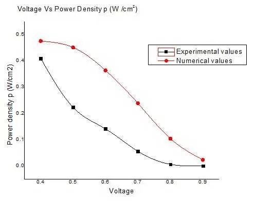
The polarization curve for serpentine 50×50 mm model for numerical and experimental values. PEM fuel cells with serpentine 50×50 mm model at 0.4V give the maximum power densities. 0.408000`W/(cm^2)`.

Conclusion:

PEMFC WITH SINGLE FLOW CHANNEL:

From the numerical analysis, the following conclusions were made. Among the four different operating pressures and five different operating temperatures, the PEM fuel cell with a single flow channel at 2.0 bar and `40^0`C gives a better performance than others.

SERPENTINE 50×50 mm MODEL:

In this project, a PEM fuel cell with 50×50 mm serpentine flow field geometry was taken into numerical as well as experimental analysis. From the above numerical comparisons, the following conclusions were made. The PEM fuel cell with a serpentine flow channel of 50×50 mm active area at an operating voltage of 0.4V gives the maximum current and power densities of 1.1860 `A/(cm^2)` & 0.4744 `W/(cm^2)` compared with other operating voltages. So, it was concluded that the 50×50 mm serpentine model gives better performance at an operating voltage of 0.4V. In future rounds, spiral flow channel cross-sections will be examined both numerically and experimentally.