NASA FILE PARSING
AIM:
PARSING OF NASA THERMODYNAMIC DATA USING MATLAB
INTRODUCTION:
Parsing or syntax analysis is the process of analyzing a string or a text into logical syntactic roles. In general, the term "parsing" refers to MATLAB reading an m-file (script or function) and translating it into an internal code which is stored in the memory. It is this "parsed" file in the memory that actually runs when we execute the code. File parsing helps in storing the calculated values in text form or any other form, it helps in the reading of information provided in any form of a file and use it to solve complex problems and giving them a graphical representation of the solution. Basically, parsing is splitting of a file into pieces of data that can be easily stored or manipulated.
In this report, we have ‘Thermodynamic data’ file provided by NASA.
Data: https://drive.google.com/file/d/1AikCHDlz9s_fu8whE81qee_GD4AyYpCP/view
Using MATLAB coding, we have to parse the data file by reading the file line by line for operation of extracting coefficient, calculating thermodynamic properties and molecular weight, etc. In the given data file, we have 53 different species like 02, CO2, N2, etc, each having 14 coefficients. These coefficients are divided like, first seven are High temperature coefficients and other seven are Low temperature coefficients, we have to find thermodynamic properties at both high and low temperatures.
COMMONLY USED COMMANDS IN MAIN PROGRAM
1) fgetl- Read line from file, removing newline characters
2) strsplit- Split string or character vector at specified delimiter
3) strfind- Find strings within other strings
4) str2double- Converts strings to double precision value
5) mkdir- Make new folder
6) cd- Change current folder
GOVERNING EQUATIONS:
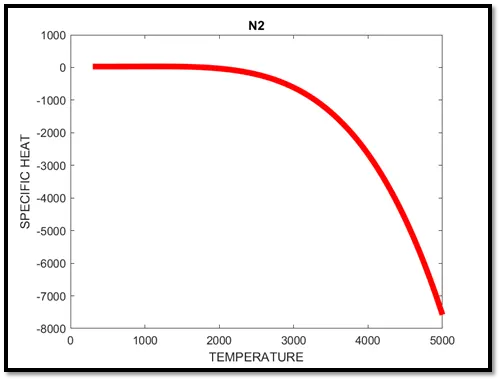
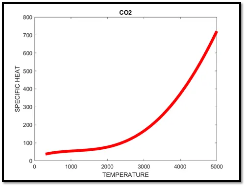
1) SPECIFIC HEAT
`(Cp)/R = a1 + a2*T + a3*T^2 + a4*T^3 + a5*T^4`
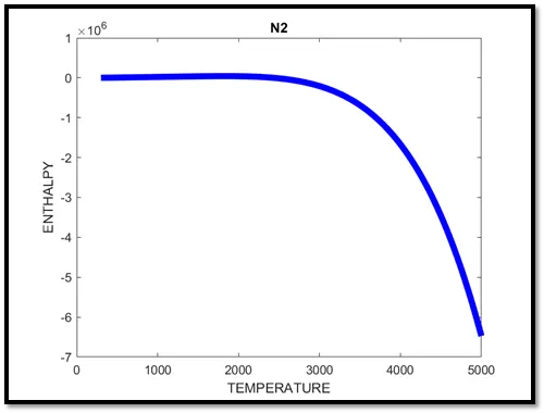
2) ENTHALPY
`H/(RT) = a1 + a2*T/2 + a3*T^3/3 + a4*T^4/4 + a5*T^5/5 + a6/T`
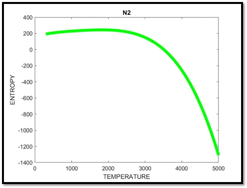
3) ENTROPY
`S/R = a1*lnT + a2*T + a3*T^2 / 2 + a3*T + a4*T^3 / 3 + a5*T^4 / 4 + a7`
Where,
Cp – Specific Heat (J / K-Kg)
H – Enthalpy (J)
S - Entropy (J / K)
R – Universal gas constant (8.314 J / mol-K)
T – Temperature (K)
a1 to a7 – High temperature
a8 to a14 – Low temperature
OBJECTIVES:
1) Write a function that extracts 14 coefficients
2) Calculate the enthalpy, entropy and specific heat of all species present in the data file.
3) Calculate molecular weight of each species and show it in command window.
4) To save all the plots as images and dump them in a separate folder for each species with suitable names.
Common commands used in starting of every program-
Clear all command for clearing workspace
Close all command for closing plots and figures in background
Clc command for clearing the command window
PROGRAM:
MATLAB PROGRAM 1- FUNCTION PROGRAM (THERMAL PROPERTIES)
%Defining the function
function [cp, h, s] = coeff_properties_func(a1,a2,a3,a4,a5,a6,a7,a8,a9,a10,a11,a12,a13,a14,T);
R = 8.314;
for i = 1:length(T)
    if T(i) < 300

        cp = (a1 + a2.*T + a3.*T.^2 + a4.*T.^3 + a5.*T.^4).*R;
        h = (a1 + (a2.*T)./2 + (a3.*T.^2)./3 + (a4.*T.^3)./4 + (a5.*T.^4)./5 + (a6./T)).*R.*T;
        s = (a1.*log(T) + a2.*T + (a3.*T.^2)./2 + (a4.*T.^3)./3 + (a5.*T.^4)./4 + a7).*R;
    else
        cp = (a8 + a9.*T + a10.*T.^2 + a11.*T.^3 + a12.*T.^4).*R;
        h = (a8 + (a9.*T)./2 + (a10.*T.^2)./3 + (a11.*T.^3)./4 + (a12.*T.^4)./5 + (a13./T)).*R.*T;
        s = (a8.*log(T) + a9.*T + (a10.*T.^2)./2 + (a11.*T.^3)./3 + (a12.*T.^4)./4 + a14).*R;
    end
end

end
Explanation:
Line1- Defining the function to calculate the thermodynamic properties- specific heat, enthalpy, entropy
Line2- Gas constant value 8.314
Line3- Assigning the value for vector ’T’ (Temperature) using for-loop
Line4- ‘If' evaluates the temperature, and executes a group of statements when the temperature is less than 300K
Line5- Defining specific heat for local low temperatures
Line6- Defining enthalpy for local low temperatures
Line7- Defining entropy for local low temperatures
Line8- ‘Else' statement is executed only when the temperature is more than 300K
Line9- Defining specific heat for local high temperatures
Line10- Defining enthalpy for local high temperatures
Line11- Defining entropy for local high temperatures
Line12- End of ‘if’ statement
Line13- End of ‘for-loop'
Line14- Closing the function
MATLAB PROGRAM 2- FUNCTION PROGRAM (MOLECULAR WEIGHT)
%Defining the function
function [molecular_weight] = mol_wei_func(name_of_species);
SPECIES = upper(name_of_species);
constituents = {'H', 'C', 'N', 'O', 'A', 'S'};
atomic_weight = [1 12 14 16 40 32];

molecular_weight = 0;
for i = 1:length(SPECIES)
    for j = 1:length(constituents)
        if strcmp(SPECIES(i),constituents(j))
            molecular_weight = molecular_weight + atomic_weight(j);
            u = j;
        end
    end

    n = str2double(SPECIES(i));
    if n > 1
        molecular_weight = molecular_weight + atomic_weight(u)*(n-1);
    end
end
fprintf('molecular_weight of %s: ',name_of_species);
fprintf('%d',molecular_weight);
fprintf(' ');
fprintf('amu');
end
Explanation:
Line1- Defining the function to calculate the molecular weight of species in the data file
Line2- Converting the string to uppercase
Line3- Defining the species elements
Line4- Atomic weight of each mentioned element in the constituents is given
Line5- Initially, molecular weight is defined as zero
Line6- Using the for-loop assigning the value for vector ‘SPECIES’
Line7- For inner loop, comparing each and every elements of species with the ’constituent’ array.
Line8- Comparing the strings, ‘constituents’ and ‘species’
Line9- Defining the molecular weight
Line10- Ending the ‘if’ statement
Line11- Ending the inner for-loop ‘j’
Line12- str2double converts the text in string to double precision values.
Line13- if statement evaluates the energy levels of the species in the data file
Line14- Defining the molecular weight if n is less than one
Line15- Ending the if statement
Line16- Ending the for-loop ‘i’
Line17,18,19&20- Command to show the molecular weight value statement with the obtained results
Line21- Closing the function
MATLAB PROGRAM 3- MAIN PROGRAM
clear all
close all
clc

% Opening the file to read
f1 = fopen('THERMO.dat','r');

% Header of the file
Header = fgetl(f1);

% Global temperature value
global_temp_line = fgetl(f1);
a1 = strsplit(global_temp_line,' ');
global_low_temp = str2double(a1{2});
global_mid_temp = str2double(a1{3});
global_high_temp = str2double(a1{4});

% Comments in the data file
comment_1 = fgetl(f1);
comment_2 = fgetl(f1);
comment_3 = fgetl(f1);

% Extracting coefficients
for i = 1:53
    line = fgetl(f1);
    species = strsplit(line,' ');
    A = species(1);
    name_of_species = char(A);

    % Local temperature values
    Local_temp_line = strsplit(line,'G');

    % Extracting from first line
    line1 = fgetl(f1);
    l1 = strfind(line1,'E');
    a1 = str2double(line1(1:(l1(1)+3)));
    a2 = str2double(line1((l1(1)+4):(l1(2)+3)));
    a3 = str2double(line1((l1(2)+4):(l1(3)+3)));
    a4 = str2double(line1((l1(3)+4):(l1(4)+3)));
    a5 = str2double(line1((l1(4)+4):(l1(5)+3)));

    %Extracting from second line
    line2 = fgetl(f1);
    l2 = strfind(line2,'E');
    a6 = str2double(line2(1:(l2(1)+3)));
    a7 = str2double(line2((l2(1)+4):(l2(2)+3)));
    a8 = str2double(line2((l2(2)+4):(l2(3)+3)));
    a9 = str2double(line2((l2(3)+4):(l2(4)+3)));
    a10 = str2double(line2((l2(4)+4):(l2(5)+3)));

    %Extracting from third line
    line3 = fgetl(f1);
    l3 = strfind(line3, 'E');
    a11 = str2double(line3(1:(l3(1)+3)));
    a12 = str2double(line3((l3(1)+4):(l3(2)+3)));
    a13 = str2double(line3((l3(2)+4):(l3(3)+3)));
    a14 = str2double(line3((l3(3)+4):(l3(4)+3)));

% Creating file to store all the plots for each species
Directory = mkdir(['D:Matlab programsNASA file parsingSPECIES1PLOTS-',name_of_species]);

% Creating array of temperature
T = linspace(global_low_temp,global_high_temp,500);

% For calculating thermodynamic function
[cp, h, s] = coeff_properties_func(a1,a2,a3,a4,a5,a6,a7,a8,a9,a10,a11,a12,a13,a14,T);

% Plotting between temperature and specific heat
figure(1)
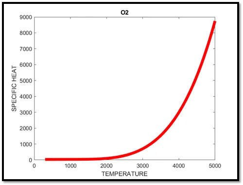
plot(T,cp,'linewidth',5,'color','r');
title(name_of_species);
xlabel('TEMPERATURE');
ylabel('SPECIFIC HEAT');

% Plotting between Temperature and enthalpy
figure(2)
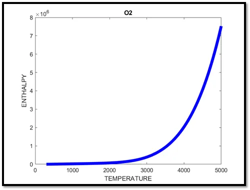
plot(T,h,'linewidth',5,'color','b');
title(name_of_species);
xlabel('TEMPERATURE');
ylabel('ENTHALPY');

% Plotting between temperature and entropy
figure(3)
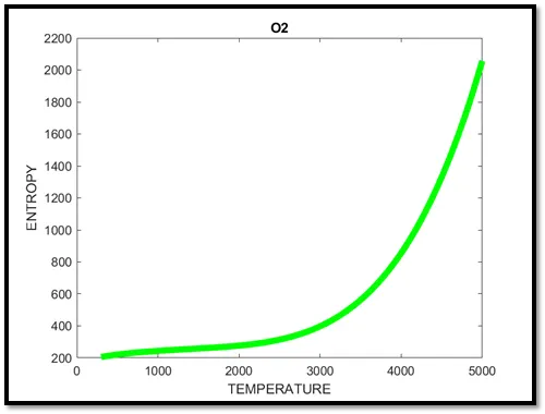
plot(T,s,'linewidth',5,'color','g');
title(name_of_species);
xlabel('TEMPERATURE');
ylabel('ENTROPY');

cd(['D:Matlab programsNASA file parsingSPECIES1PLOTS-',name_of_species]);

% Saving the plots
saveas(1,'specific heat.png');
saveas(2,'enthalpy.png');
saveas(3,'entropy.png');

% Changing the directory for calculating molecular weight
cd('D:Matlab programsNASA file parsing');
[molecular_mass] = mol_wei_func(name_of_species);

end
fclose(f1)
Explanation:
Line1- Opening the data file and reading it
Line2- For reading header of the file
Line3- Reading the global temperature values as a string
Line4- The string of global temperature value is split by delimiter ‘ ‘, i.e. space.
Line5- The global temp low temperature as a string gets converted into an individual number value.
Line6- The global temp mid temperature as a string gets converted into an individual number value.
Line7- The global temp high temperature as a string gets converted into an individual number value.
Line8,9&10- Starting three comments after the header and global temperature of the data file.
Line11- ‘For-loop' to extract 14 coefficients from all 53 species present in the data file.
Line12- The sixth line in the data file is read for first iteration and stored in the variable called ‘line’
Line13- The sixth line is split by delimiter ‘ ‘ (space) and is converted into a cell array
Line14- First element in cell array is stored in variable ‘A’
Line15- Converting cell array into character array
Line16- The second line under the species are read and stored in ‘line1’
Line17- The second line is in string format and the position of ‘E’ is calculated
Line18,19,20,21&22- First five coefficients are calculated
Line23- The third line under the species are read and stored in line2
Line24- The third line is in string format and the position of ‘E’ is calculated
Line25,26,27,28&29- The next five coefficients are calculated, i.e. from 6th to 10th
Line30- The fourth line under the species are read and stored in line3
Line31- The fourth line is in string format and the position of ‘E’ is calculated
Line32- Creating a file path and a folder name ‘SPECIES’
Line33- Creating temperature array
Line34- Calling the function for calculating the thermodynamic properties of the species, ‘specific heat, enthalpy, entropy’
Line35&36- Creating figure (1) window to show the plotting of Temperature vs Specific heat
Line37- Labelling x-axis ‘Temperature’
Line38- Labelling y-axis ‘Specific Heat’
Linne39&40- Creating figure (2) window to show the plotting of Temperature vs Enthalpy
Line41- Labelling x-axis ‘Temperature’
Line42- Labelling y-axis ‘Enthalpy’
Line43&44- Creating figure (3) window to show the plotting of Temperature vs Entropy
Line45- Labelling x-axis ‘Temperature’
Line46- Labelling y-axis ‘Entropy’
Line47- Statement navigates the program to directory and the folder ‘SPECIES’
Line48- The plots of Temperature vs Specific heat are being saved in .png format
Line49- The plots of Temperature vs Enthalpy are being saved in .png format
Line50- The plots of Temperature vs Entropy are being saved in .png format
Line51&52- Changing the directory and calling the function for calculating the molecular weight of the species present in the data file
Line53- Ending the ‘for-loop'
Line54- Closing the ‘THERMO.dat’ file
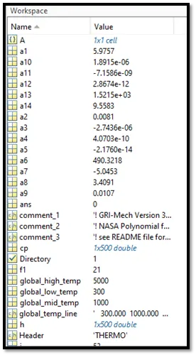
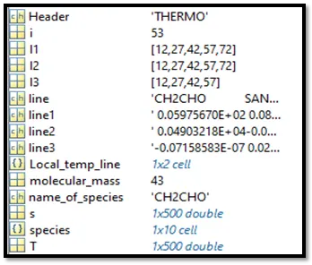
Fig.1. Output Values
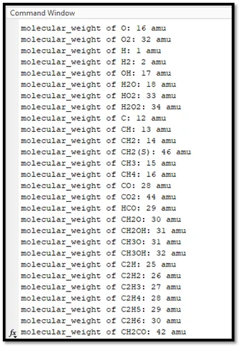
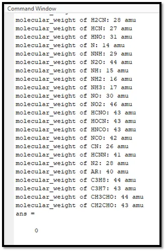
Fig.2. Molecular Weights of Species
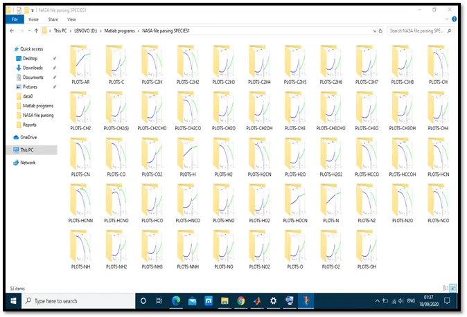
Fig.3. Folder path for plots of all the species in the data file
PLOTS:
1) For O2-
2) For N2-
3) For CO2-
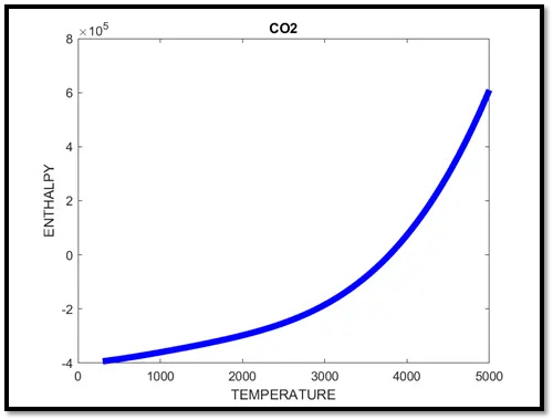
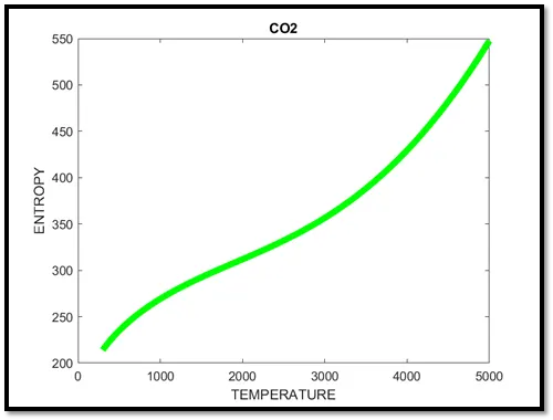
CONCLUSION: WE HAVE STUDIED ABOUT PARSING OF DATA FILE USING MATLAB, GETTING A CLEAR UNDERSTANDING ABOUT READING OF A DATA FILE IN MATLAB FOR VARIOUS APPLICATIONS. WE UNDERSTOOD THE IMPORTANCE OF READING OF DATA AND SIMPLIFYING IT FOR BETTER UNDERSTANDING BY GIVING THE DATA A GRAPHICAL REPRESENTATION.
REFRENCES:
2.https://en.wikipedia.org/wiki/Parsing#Computer_languages
3.https://in.mathworks.com/help/matlab/matlab_prog/parse-function-inputs.html