GENETIC ALGORITHM

AIM:

TO UNDERSTAND GENETIC ALGORITHM AND WRITE CODE FOR OPTIMIZING THE STALAGMITE FUNCTION AND FIND ITS GLOBAL MAXIMA

INTRODUCTION:

GENETIC ALGORITHM

A genetic algorithm (GA) is a method for solving both constrained and unconstrained optimization problems based on a natural selection process that mimics biological evolution. The algorithm repeatedly modifies a population of individual solutions. At each step, the genetic algorithm randomly selects individuals from the current population and uses them as parents to produce the children for the next generation. Over successive generations, the population "evolves" toward an optimal solution.

Genetic algorithm (GA) is the process of natural selection that belongs to the larger class of evolutionary algorithm (EA). Genetic algorithms are commonly used to generate high-quality solutions to optimization and search problems by relying on biologically inspired operators such as mutation, crossover and selection.

The in-built solver for genetic algorithm in MATLAB is ‘ga’.

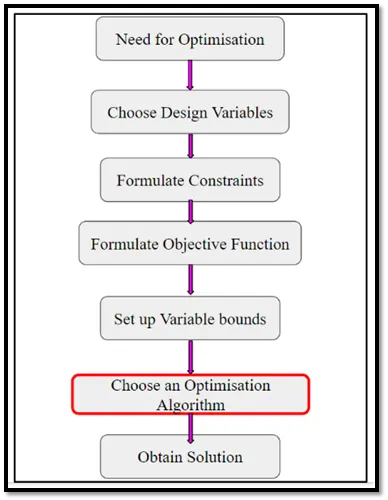
Fig.1. Optimization process

• How does (GA) works?

The following outline summarizes how the genetic algorithm works:

1. The algorithm begins by creating a random initial population.
2. The algorithm then creates a sequence of new populations. At each step, the algorithm uses the individuals in the current generation to create the next population. To create the new population, the algorithm performs the following steps:
3. Scores each member of the current population by computing its fitness value. These values are called the raw fitness scores.
4. Scales the raw fitness scores to convert them into a more usable range of values. These scaled values are called expectation values.
5. Selects members, called parents, based on their expectation.
6. Some of the individuals in the current population that have lower fitness are chosen as elite. These elite individuals are passed to the next population.
7. Produces children from the parents. Children are produced either by making random changes to a single parent—mutation—or by combining the vector entries of a pair of parents—crossover.
8. Replaces the current population with the children to form the next generation.
9. The algorithm stops when one of the stopping criteria is met. These stopping constraints are:

a.Generations- Specifies the no. of generations that MATLAB has to produce.

b.Time- The GA will stop running for a time period set by user.

c.Tolerance- This a strong stopping criterion, specifies convergence limit between two populations and when they differ by less than this amount then the algorithm will stop.

• What is the usage of (GA)?

(GA) is used to find global minima, if the problem has large data-set having random probability distribution or pattern with complex constraints to apply then finding global minima using the standard optimization (i.e. differentiation) is complex and tedious task to perform. Thus (GA) genetic algorithm is used to solve problems that are not well suited for standard optimization algorithms, including problems in which the objective function is discontinuous, nondifferentiable, stochastic, or highly nonlinear. It can solve smooth and non-smooth optimization problems with any type of constraints. It is a stochastic and population-based algorithm that searches randomly by mutation, crossover among population members.

It is frequently used to solve optimization problems, in research, and in machine learning, neural networks, image processing, etc.

Genetic Algorithm Terminology

1. Fitness function- It takes the solution as input and produces the suitability of the solution as the output. This evaluates how close the solution is to the optimal solution of the desired problem.
2. Individual- An individual is any point to which you can apply the fitness function. The value of the fitness function for an individual is its score. An individual is sometimes referred to as a genome and the vector entries of an individual as genes.
3. Population- It is the number of sample data points taken to perform the genetic algorithm operation.
4. Generation- At each iteration, the genetic algorithm performs a series of computations on the current population to produce a new population. Each successive population is called a new generation.
5. Diversity- It refers to the average distance between individuals in a population. A population has high diversity if the average distance is large; otherwise it has low diversity. In the following figure, the population on the left has high diversity, while the population on the right has low diversity. It is essential to the genetic algorithm because it enables the algorithm to search a larger region of the space.
6. Parents and children- To create the next generation, the genetic algorithm selects certain individuals in the current population, called parents, and uses them to create individuals in the next generation, called children. Typically, the algorithm is more likely to select parents that have better fitness values.

SYNTAX OF GA

• The syntax of ga(function, n_variables) will give the local unconstrained minimum, to the objective function. Here n_variables are the number of independent variables in the function.
• ga(@stalagmite_function, variables, A, b) finds a local minimum x to function, subject to linear inequalities Ax ≤ b.
• ga(@stalagmite_function, A, b, Aeq, beq) finds a local minimum, subject to linear inequalities Aeq*x = beq and Ax ≤ b.
• ga(@stalagmite_function, variables, A, b, Aeq, beq, X, Y) defines the set of lower and upper bounds on the design variables in terms of column matrix.
• ga(@stalagmite_function, variables, A, b, Aeq, beq, X, Y, non_lin, int, options), finds a minimum subject to nonlinear constraints, options can contain several initializations like population size, fitness scaling function, etc.

GOVERNING EQUATIONS:

STALAGMITE FUNCTION

f(x,y) = f1x . f2y . f2x . f2y

Where,

The function has four components:

1) 2 sine components in each of the axis direction

f1x = (sin(5.1πx + 0.5))^6

f1y = (sin(5.1πy + 0.5))^6

2) 2 normal gaussian distribution in each of the axis direction

f2x = exp [ -4ln(2) . (x –0.667)^2 / 0.64 ]

f2y = exp [ -4ln(2) . (y – 0.667)^2 / 0.64]

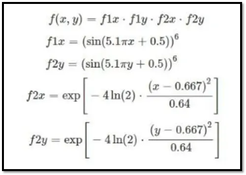
Fig.2. Stalagmite function

OBJECTIVES:

1. To optimize the stalagmite function

1. To determine Global Maxima of the function

Common commands used in starting of every program-

Clear all command for clearing workspace

Close all command for closing plots and figures in background

Clc command for clearing the command window

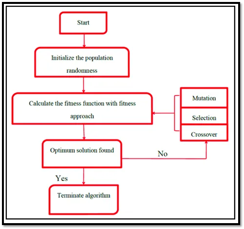
Fig.3. Flowchart for GA

PROGRAM:

MATLAB PROGRAM 1- FUNCTION PROGRAM

% Defining the function 
function [f] = stalagmite_func(input_vector)
  
% Segregating the inputs
x = input_vector(1);
y = input_vector(2);

% Computing the stalagmite function
f1x_1 = sin(5.1*pi*x + 0.5).^6; 
f1y_1 = sin(5.1*pi*y + 0.5).^6;

f2x_1 = exp ( -4.*log(2) * (x - 0.6667).^2 / 0.64);
f2y_1 = exp ( -4.*log(2) * (y - 0.6667).^2 / 0.64); 
 
% Returninng the value
f = (-1) *  f1x_1 * f1y_1 * f2x_1 * f2y_1;
end

Explanation:

Line1- Function is created that defines the input variable as a two-dimensional matrix (input_vector) and then produce a value at specified x and y.

Line2&3- Defining x and y

Line4&5- Defining the sine components

Line6&7- Defining the normal gaussian distribution

Line8- Defining the stalagmite function, x and y values will be return as scaler value corresponding to the value of stalagmite function at that point with a negative sign i.e. returning negative of original value hence (–1) is multiplied.

Line9- Closing the function

MATLAB PROGRAM 2- MAIN FUNCTION (UNBOUNDED)

clear all 
close all
clc

% Defining search space
x = linspace(0,0.6,150);
y = linspace(0,0.6,150);

% Number of test cases
num_cases = 100;

% Creating 2D mesh
[xx, yy] = meshgrid(x,y);

% Evaluating stalagmite function
for i = 1:length(xx);
  for j = 1:length(yy);
    input_vector(1) = xx(i,j);
    input_vector(2) = yy(i,j);
    f(i,j) = (-1) * stalagmite_func(input_vector);
  end
  end

% Starting the time
tic
% Runing ga algorithm for unbounded
for i = 1:num_cases;
  [inputs, output_1(i)] = ga(@stalagmite_func, 2);
  % Extracting co-ordinates
  case1_x(i) = inputs(1);
  case2_y(i) = inputs(2);
end
% Ending the time
study_time = toc

% Plotting and labeling for iterations wrt minimum value
figure(1);
set(gcf,'position' ,[100,100,1000,1000]); 
plot(-output_1);
xlabel('Number of iteration');
ylabel('Min. value to algorithm');
title('Min. value at different iterations');
grid on;
grid minor;
set(gca,'fontsize',15);

% Plotting and labeling of stalagmite function
figure(2);
set(gcf,'position' ,[100,100,1000,1000]); 
surfc(xx,yy,f);
hold on
plot3(case1_x, case2_y, -output_1,'marker', '*', 'markersize',6,'linew',3);
xlabel('X-value');
ylabel('Y-value');
zlabel('Function value');
title('Unbounded inputs');
shading interp;
axis tight;
colormap jet;
colorbar;
set(gca,'fontsize',20);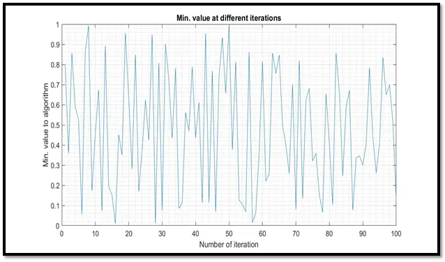

Fig.4. Min. Value at different iterations

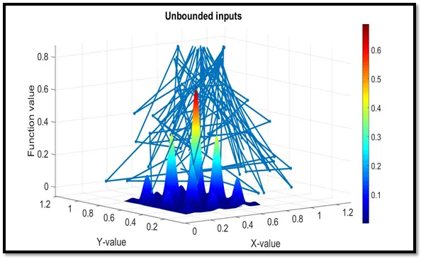
Fig.5. Unbounded inputs (Max. Value at the top of the function)

Explanation:

Line1&2- Defining the search space, creating x and y vector in x and y direction

Line3- No. Of tests

Line4- Creating 2D grid coordinates based on vector x and y

Line5- Assigning the value at each grid point using for-loop for vector ‘xx’

Line6- For inner loop, assigning the value for vector ’yy’

Line7,8&9- Defining the input vector, computing the values at defined grid point and storing it in a variable ‘f’

Line10&11- End for-loop for i and j

Line12- Starting the time, ‘tic’

Line13&14- Assigning the ‘ga’ to run 100 times where all the results are stored in output_1 by calling the stalagmite function

Line15,16&17- Extracting the coordinates where all the minimum values are stored in ‘case1_x’ and ‘case2_y’, ending the for-loop

Line18- Ending the time, ‘toc’

Line19- Creating figure(1) window to show the plotting of output values is done with respect to different iterations

Line20- Defining the object graphics properties, ‘gcf’ returns the current figure handle

Line21- Plotting the output

Line22,23&24- Labelling x-axis and y-axis, title for the plot

Line25- To show the grid lines

Line26- To make the appearance of the grid lines smooth and clean

Line27- Returns the current axis for the current figure

Line28- Creating figure(2) window to show the plotting of stalagmite function

Line29- Defining the object graphics properties, ‘gcf’ returns the current figure handle

Line30- Creating 3D surface plot

Line31- Retains the plot in current axis

Line32- Plotting the coordinates in 3D space

Line33,34,35&36- Labelling of x,y and z axis, giving title to the plot

Line37- It varies the color in each line segment and face by interpolating the colormap index or true color value across the line or face.

Line38- Fills the white space

Line39 - Sets the colormap of current figure to one of its predefined colormaps.

Line40- Returns the current axis for the current figure

The runtime stimulation-

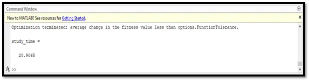
In the graph obtained shows the optimization by MATLAB, the maximum values are spread across all over the plot, this is because the search space is not defined. Hence, the second study case for optimization...

MATLAB PROGRAM 3- BOUNDED FUNCTION (LIMITED SEARCH SPACE BETWEEN 0 TO 0.5)

% Bounded inputs
close all 
clear all
clc

% Defining search space
x = linspace(0,0.6,150);
y = x;

% Number of test cases
num_cases = 100;

% Creating 2D mesh
[xx, yy] = meshgrid(x,y);

% Evaluating stalagmite function
for i = 1:length(xx);
  for j = 1:length(yy);
    input_vector(1) = xx(i,j);
    input_vector(2) = yy(i,j);
    f(i,j) = (-1) * stalagmite_func(input_vector);
  end
end
  
% Starting the time
tic;
% Runing ga algorithm for bounded inputs
for i = 1:num_cases;
  [inputs, output_2(i)] = ga(@stalagmite_func, 2,[],[],[],[],[0;0],[0.5;0.5]);
  % Extracting co-ordinates
  case1_x(i) = inputs(1);
  case2_y(i) = inputs(2);
end
% Ending the time
end_time = toc;

% Plotting the output values for minimum
  figure(3);
  set(gcf,'position' ,[100,100,1000,1000]); 
  plot(-output_2)
  xlabel('Number of iteration');
  ylabel('Min. value for GA');
  title('Min. value at different iterations for search space 0 to 0.5 ');
  grid on;
  grid minor;
  
  % Plotting stalagmite function
  figure(4);
  surfc(xx,yy,f);
  hold on;
  plot3(case1_x, case2_y, -output_2,'marker', '*', 'markersize',8,'linew',4);
  shading interp;
  axis tight;
  title('Max.value at the top of the function for search space 0 to 0.5');
  xlabel('X-value');
  ylabel('Y-value');
  zlabel('Function value');
  rotate3d on;
  colorbar;
  colormap jet;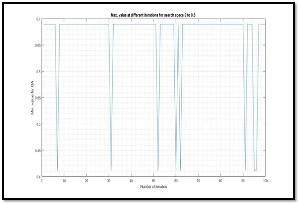

Fig.6. Bounded inputs (Max. Value at different iterations for search space 0 to 0.5)

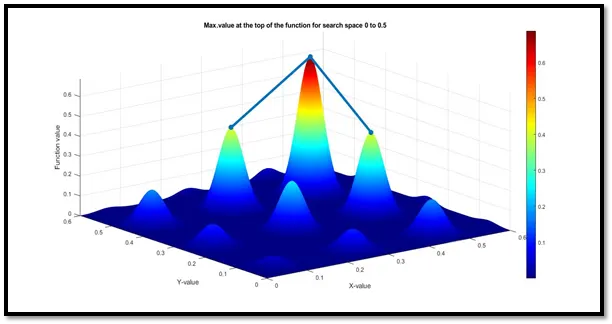
Fig.7. Bounded inputs (Max. Value at the top of the function)

Explanation:

Line1&2- Defining the search space, creating x and y vector in x and y direction

Line3- No. Of tests

Line4- Creating 2D grid coordinates based on vector x and y

Line5- Assigning the value at each grid point using for-loop for vector ‘xx’

Line6- For inner loop, assigning the value for vector ’yy’

Line7,8&9- Defining the input vector, computing the values at defined grid point and storing it in a variable ‘f’

Line10&11- End for-loop for i and j

Line12- Starting the time, ‘tic’

Line13&14- Assigning the ‘ga’ to run 100 times where all the results are stored in output_1 by calling the stalagmite function having defined search space for optimization between 0 to 0.5. The brackets ([]) in the function removes any linear inequality constraints.

Line15,16&17- Extracting the coordinates where all the minimum values are stored in ‘case1_x’ and ‘case2_y’, ending the for-loop

Line18- Ending the time, ‘toc’

Line19- Creating figure(3) window to show the plotting of output values is done with respect to different iterations

Line20- Defining the object graphics properties, ‘gcf’ returns the current figure handle

Line21- Plotting the output

Line22,23&24- Labelling x-axis and y-axis, title for the plot

Line25- To show the grid lines

Line26- To make the appearance of the grid lines smooth and clean

Line27- Returns the current axis for the current figure

Line28- Creating figure(4) window to show the plotting of stalagmite function

Line29- Defining the object graphics properties, ‘gcf’ returns the current figure handle

Line30- Creating 3D surface plot

Line31- Retains the plot in current axis

Line32- Plotting the coordinates in 3D space

Line33,34,35&36- Labelling of x,y and z axis, giving title to the plot

Line37- It varies the color in each line segment and face by interpolating the colormap index or true color value across the line or face.

Line38- Fills the white space

Line39 - Turns on rotate mode and enables rotation in all direction.

Line40- Sets the colormap of current figure to one of its predefined colormaps.

It can be seen in fig.6 that by limiting the search space, we have fewer oscillations compared to with no constraints. But this method for optimization won’t work if we don’t have effective search space thus for finding global maxima, we use altering population size method...

MATLAB PROGRAM 4- BOUNDED FUNCTION (ALTERED POPULATION SIZE FOR GLOBAL MAXIMA)

% Bounded inputs with altered population size
options = optimoptions('ga');
options = optimoptions(options,'PopulationSize',500);

% Starting the time
tic;

% % Runing ga algorithm for bounded inputs
for i = 1:num_cases;
  [inputs, output_3(i)] = ga(@stalagmite_func, 2,[],[],[],[],[0;0],[0.5;0.5],[],[],options);
  % Extracting co-ordinates
  case1_x(i) = inputs(1);
  case2_y(i) = inputs(2);
end
% Ending the time
end_time = toc;

% Plotting output values
figure(5);
set(gcf,'position' ,[100,100,1000,1000]); 
  plot(-output_3)
  xlabel('Number of iteration');
  ylabel('Min. value for GA');
  title('Max. value at different iterations for search space 0 to 0.5 ');
  grid on;
  grid minor;
  
  % Plotting stalagmite function
  figure(6);
  surfc(xx,yy,f);
  hold on;
  plot3(case1_x, case2_y, -output_3,'marker', '*', 'markersize',8,'linew',4);
  shading interp;
  axis tight;
  title('Global maxima from altered population size');
  xlabel('X-value');
  ylabel('Y-value');
  zlabel('Function value');
  rotate3d on;
  colorbar;
  colormap jet;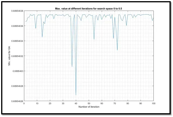

Fig.8. Bounded inputs (Altered population size)

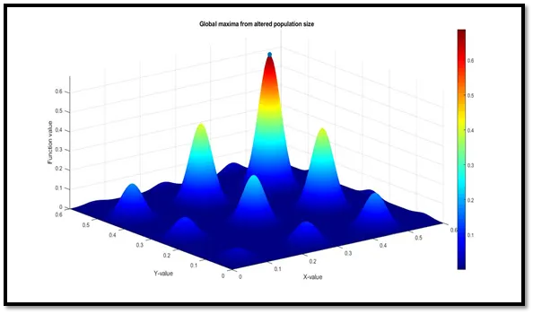
Fig.9. Bounded inputs (Global maxima)

Explanation:

Line1- Initializing optimum options, returns the default options for ‘ga’

Line2- Returns the options with a defined population size 500. The population size plays an important role in the convergence of the solution.

Line3- Starting the time

Line4&5- Assigning the ‘ga’ to run 100 times where all the results are stored in output_1 by calling the stalagmite function having defined search space for optimization between 0 to 0.5. The brackets ([]) in the function removes any linear inequality.

Line6,7&8- Extracting the coordinates where all the minimum values are stored in ‘case1_x’ and ‘case2_y’, ending the for-loop

Line9- Ending the time, ‘toc’

Line10- Creating figure(5) window to show the plotting of output values is done with respect to different iterations

Line11- Defining the object graphics properties, ‘gcf’ returns the current figure handle

Line12- Plotting the output

Line13,14&15- Labelling x-axis and y-axis, title for the plot

Line16- To show the grid lines

Line17- To make the appearance of the grid lines smooth and clean

Line18- Creating figure(6) window to show the plotting of stalagmite function

Line19- Creating 3D surface plot

Line20- Retains the plot in current axis

Line21- Plotting the coordinates in 3D space

Line22- It varies the color in each line segment and face by interpolating the colormap index or true color value across the line or face.

Line23- Fills the white space

Line24,25,26&27- Labelling of x,y and z axis, giving title to the plot

Line28- Turns on rotate mode and enables rotation in all direction.

Line29- Showing the color scale

Line30- Sets the colormap of current figure to one of its predefined colormaps.

Here, we get an exact solution i.e global maxima (a single point) at the top of the function. It is observed that with increase in population size, we get improved convergence, i.e. with higher population, genetic mutation has higher probability to produce offsprings with best genes over a period of time.

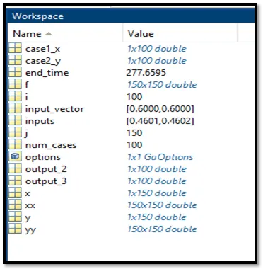
Fig.10. Workspace depicts input and output

CONCLUSION: WE HAVE STUDIED GENETIC ALGORITHM AND LEARNED ABOUT THE THEORY OF EVOLUTION AND ITS IMPORTANCE WHICH HELPS IN PREDICTION OF GENETIC MUTATION POSSIBILITIES. GA IN MATLAB HELP US TO FIND THE LOCAL AND GLOBAL MINIMAS WHICH HELPS IN ENGINEERING LEVEL OPTIMIZATION FOR PERFECT SOLUTION AND GIVING THE VISUAL CONTEXT OF THE SOLUTION.

REFRENCES:

1.skill-lync.freshdesk.com/support/solutions/articles/43000584189-genetic-algorithm-explained-

2.https://in.mathworks.com/help/gads/examples/genetic-algorithm-options.html

3.https://in.mathworks.com/help/gads/how-the-genetic-algorithm-works.html

4.https://en.wikipedia.org/wiki/Genetic_algorithm