SOLVING COUPLED DIFFERENTIAL EQUATIONS NUMERICALLY BY MULTIVARITE NEWTON RAPHSON METHOD USING BACKWARD DIFFERENCE(IMPLICIT) SCHEME IN PYTHON

Aim :

Solving coupled ODE's using multivariate newton raphson method and by implicit formulation

Introduction :

In many areas of engineering especially in combustion simulations coupled ODE's are to be solved and solving these equations analytically is not possible so these equations are solved by a numerical integration technique called Newton raphson method

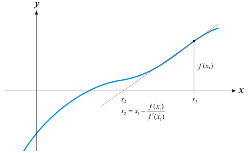
The idea is to start with an initial guess which is reasonably close to the true root and then to approximate the function by its tangent line using calculus and finally to compute the x-intercept of its tangent line by elementary algebra

The coupled Differential equations which are to be solved are

`frac{dy_1}{dt}=-0.04y_1 + 10^4y_2y_3`

`frac{dy_2}{dt} = 0.04y_1 +10^4y_2y_3 - 3*10^7*y_2^2`

`frac{dy_3}{dt} = 3*10^7*y_2^2`

Initial condition :

`y_1[0] = 1, y_2[0] = 0, y_3[0] = 0`

Applying backward differentiation scheme (implicit scheme)

`frac{y_1^n - y_1^(n-1)}{trianglet}=-0.04y_1^n + 10^4*y_2^n.y_3^n`

`frac{y_2^n - y_2^(n-1)}{trianglet} = 0.04y_1^n - 10^4y_2^ny_3^n - 3*10^7(y_2^n)^2`

`frac{dy_3}{dt} = 3*10^7*(y_2^n)^2`

Multivarient Newton raphson method :

`f_1^n =y_1^n +trianglet(0.04y_1^n -10^4y_2^ny_3^n) - y_1^(n-1) = 0`

`f_2^n = y_2^n -trianglet(0.04y_1^n -10^4y_2^ny_3^n-3*10^7(y_2^n)^2)-y_2^(n-1) =0`

`f_3^n = y_3^n -trianglet(3*10^7(y_2^n)^2)-y_3^(n-1) = 0`

Jacobian matrix :

There are three equations and three variables

`J=[[frac{partialf_1^n}{partialy_1^n},frac{partialf_1^n}{partialy_2^n},frac{partialf_1^n}{partialy_3^n}],[frac{partialf_2^n}{partialy_1^n},frac{partialf_2^n}{partialy_2^n},frac{partialf_2^n}{partialy_3^n}],[frac{partialf_3^n}{partialy_1^n},frac{partialf_3^n}{partialy_2^n},frac{partialf_3^n}{partialy_3^n}]]`

`y(n_(ew))^n =y_(old)^n + alpha[(J^-1)F]^n`

`F =[[f_1],[f_2],[f_3]]`

Code structure :

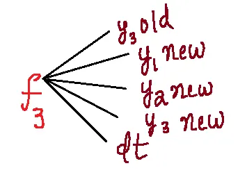
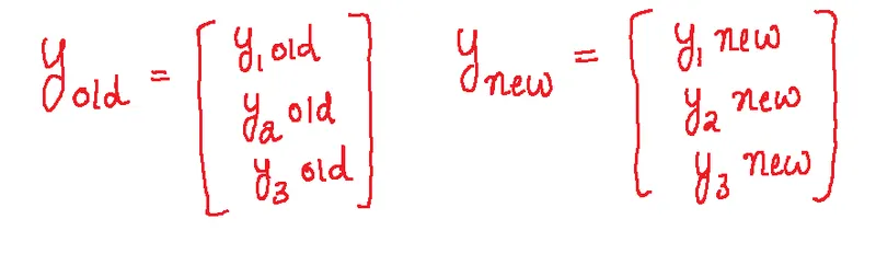
python code :

'''
Program to solve system of ODE's using multivariate Newton raphson solver

d(y1)/dt= -0.04 y1 + 10^4 y2y3
d(y2)/dt= 0.04 y1 - 10^4 y2y3 - 3*10^7 y2^2
d(y3)/dt= 3*10^7 y2^2

Author : Harshith Rajamahanti

'''
import numpy as np
import matplotlib.pyplot as plt
from numpy.linalg import inv 
from numpy import array

# Defining the functions for solving ODE's 

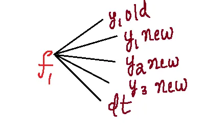
def f1(y1_old,y1_new,y2_new,y3_new,dt):
	
	# First non linear equation 
	return y1_old-dt*(0.04*y1_new - 1e4*y2_new*y3_new)-y1_new

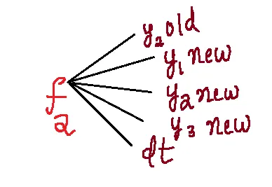
def f2(y2_old,y1_new,y2_new,y3_new,dt):
	
	# 2nd non linear equation 
	return y2_old+dt*(0.04*y1_new - 1e4*y2_new*y3_new -3e7*pow(y2_new,2))-y2_new

def f3(y3_old,y1_new,y2_new,y3_new,dt):
	
	# 3rd non linear equation 
	return y3_old+dt*(3e7*pow(y2_new,2))-y3_new

def jacobian(y_new,y_old,dt):
	
	dy=1e-5 
	j=np.zeros((3,3))

	# Row 1

	j[0,0]=(f1(y_old[0],y_new[0]+dy,y_new[1],y_new[2],dt)-f1(y_old[0],y_new[0],y_new[1],y_new[2],dt))/dy
	j[0,1]=(f1(y_old[0],y_new[0],y_new[1]+dy,y_new[2],dt)-f1(y_old[0],y_new[0],y_new[1],y_new[2],dt))/dy
	j[0,2]=(f1(y_old[0],y_new[0],y_new[1],y_new[2]+dy,dt)-f1(y_old[0],y_new[0],y_new[1],y_new[2],dt))/dy

	# Row 2

	j[1,0]=(f2(y_old[1],y_new[0]+dy,y_new[1],y_new[2],dt)-f2(y_old[1],y_new[0],y_new[1],y_new[2],dt))/dy
	j[1,1]=(f2(y_old[1],y_new[0],y_new[1]+dy,y_new[2],dt)-f2(y_old[1],y_new[0],y_new[1],y_new[2],dt))/dy
	j[1,2]=(f2(y_old[1],y_new[0],y_new[1],y_new[2]+dy,dt)-f2(y_old[1],y_new[0],y_new[1],y_new[2],dt))/dy

	# Row 3

	j[2,0]=(f3(y_old[2],y_new[0]+dy,y_new[1],y_new[2],dt)-f3(y_old[2],y_new[0],y_new[1],y_new[2],dt))/dy
	j[2,1]=(f3(y_old[2],y_new[0],y_new[1]+dy,y_new[2],dt)-f3(y_old[2],y_new[0],y_new[1],y_new[2],dt))/dy
	j[2,2]=(f3(y_old[2],y_new[0],y_new[1],y_new[2]+dy,dt)-f3(y_old[2],y_new[0],y_new[1],y_new[2],dt))/dy

	return j

# Constructing time array 

t_start=0
t_stop=500
dt=0.5
n=(t_stop-t_start)/dt + 1
t=np.linspace(t_start,t_stop,int(n))

y_old=np.zeros((3,1))
y_old[0]=1
y_new=np.zeros((3,1))

# column vector for F 
F=np.copy(y_old)

# parameters for newton raphson solver

alpha=1.1
tol=1e-7
error=9e9
iter=0

y1=[]
y1.append(1)
y2=[]
y2.append(0)
y3=[]
y3.append(0)

for i in range(1,len(t)):
	
	y1_old=y_old[0]
	y2_old=y_old[1]
	y3_old=y_old[2]
	y_old_temp=np.copy(y_old)

	while error>=tol:

		jac=jacobian(y_new,y_old,dt)
		F[0]=f1(y1_old,y_old_temp[0],y_old_temp[1],y_old_temp[2],dt)
		F[1]=f2(y2_old,y_old_temp[0],y_old_temp[1],y_old_temp[2],dt)
		F[2]=f3(y3_old,y_old_temp[0],y_old_temp[1],y_old_temp[2],dt)

		y_new=y_old_temp-alpha*(np.matmul(inv(jac),F))
		error=np.max(np.abs(y_new-y_old_temp))
		y_old_temp=y_new
		iter=iter+1

	y_old=y_new

	y1.append(y_new[0])
	y2.append(y_new[1])
	y3.append(y_new[2])

	log_message=' Time = {0} sec , iterations = {1} , y1 = {2} , y2 = {3} , y3 = {4}'.format(round(t[i],5),iter,y_new[0],y_new[1],y_new[2])

	print(log_message)

	iter=0
	error=9e9

plt.plot(t,y1,color='blue')
plt.plot(t,y2,color='red')
plt.plot(t,y3,color='black')
plt.xlabel('Time in sec')
plt.ylabel('Variable')
plt.legend(['y1','y2','y3'])
plt.title('Multivariate newton raphson solution for dt = '+ str(dt) +' sec')
plt.show()

Code explanation :

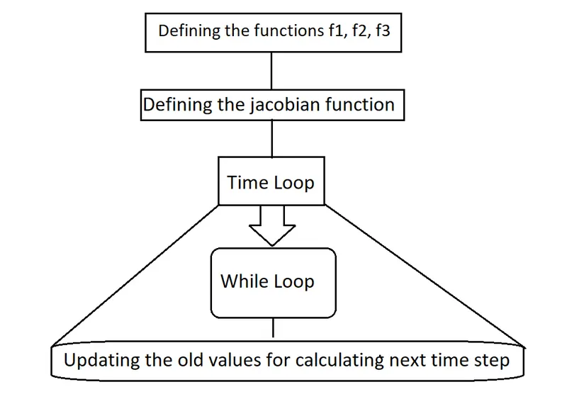
1. At first f1 f2 f3 and jacobian functions are defined
2. Time array is constructed and initial conditiions are applied
3. Initial guess values and parameters for newton raphson solver is taken
4. for loop indicates time loop and while is for newton raphson solution
5. later the values of y are updated for the next time step
6. The results are plotted

Output :

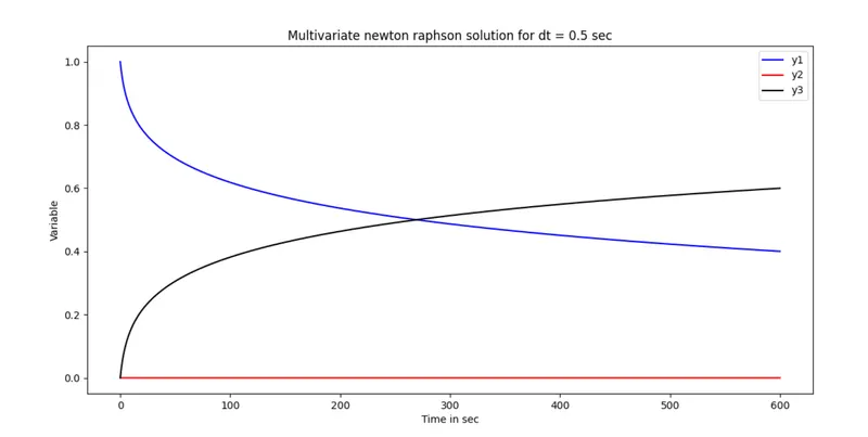
for dt =0.5

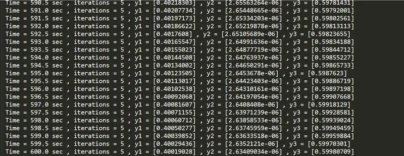
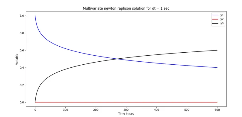
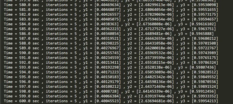
for dt = 1 sec

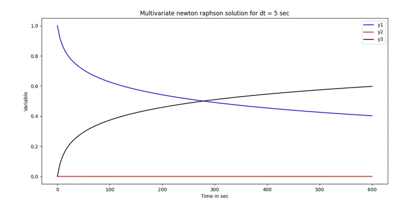
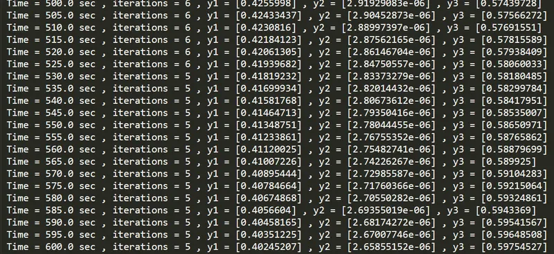
for dt = 5 sec

Conclusion :

1. For all time steps the graph has not changed so by implementing backward difference schemes (implicit scheme) the solution doesn't blown up.
2. From the graph it can be observed that y1 decrease with increase in time which resembles reactants and y3 increases with increase in time which resembles products and y2 doesnot change wrt to time.