Modelling, Simulation and Validation Of Fuel Cell Vehicle Toyota Mirai For Performance and Efficiency

Abstract

According to the energy crisis that the world faces, the community needs solutions for this problem, hydrogen fuel cells are a promising one like option to generate clean energy and solve this crisis. During the last few years of the twentieth century, people have enhanced the interest to expand the use of fuel cell technology. Environmental concerns about global warming and the need to reduce carbon dioxide (CO2) emissions provided the stimulus to seek ways of improving energy conversion efficiency. As this technology is still growing and in research, creating a vehicle powered by fuel cells and tuning it to our needs would cost us a lot. Hence, a computer simulation is done, and the system's outcome is seen before putting the system into actual production. In this report, we build a mathematical model of the vehicle, assume a standard drive cycle needed for simulation, and get the fuel economy and performance parameters as the output at the end of the simulation as the result.

Introduction & Background

1.1. Introduction

Conventional power system is facing problems like gradual depletion of fossil fuel, poor energy efficiency, and environmental pollution around the world. To overcome the above problems, non-conventional/renewable energy sources like natural gas, biogas, wind power, solar photovoltaic cells, and fuel cells can be used. The fuel cell is an electrochemical device that converts chemical energy into electrical energy and used as clean power generators. The system does not emit CO2 and NO x per kilowatt of power generated, so no air pollution occurs and only water is obtained as a by-product from the fuel cell. As there are no moving parts, the system is almost free from noise and vibration, also the robust and low maintenance design makes it suitable for both urban and suburban locations. Electrical efficiencies of fuel cells lie between 36% to 60% depending upon the type and system configuration. By using conventional heat recovery equipment and reusing the unused hydrogen in the fuel cell, overall efficiency can be enhanced to 85%.

To satisfy this need, in recent years, many automotive companies and people in their workshops have been developing vehicles, propelled by electric motors powered by energy supplied by the fuel cells. Although this technology is very expensive at present, it is thought that the price will decrease in the future with increasing demand. With the growing cost of oil and concern about global warming, people are becoming interested in cleaner, more fuel-efficient vehicle engines powered by biofuels or hydrogen, or by alternative energy technologies like batteries, hybrids, and fuel cells. And given the rising cost of electricity and reliability issues with the power distribution system, people will soon be demanding cleaner, alternative energy sources to power heat and cool their homes. An ideal technology to do just this is one of the same technologies being developed for fuel cell-powered cars.

A Fuel Cell is an electrochemical energy converter that converts the fuel's chemical energy directly into DC electricity. Photon Exchange Membrane (PEM) fuel cell consists of a membrane that acts as an electrolyte which is squeezed between the two porous, electrically conductive electrodes. These electrodes are typically made out of carbon cloth or carbon fiber paper. At the between the porous electrode and the polymer membrane, there is a layer with catalyst particles, typically platinum supported on carbon. Electrochemical reactions happen at the surface of the catalyst at the interface between the electrolyte and the membrane. Hydrogen, which is fed on one side of the membrane splits into its primary constituents
protons and electrons. Each hydrogen atom consists of one electron and one proton. Protons travel through the membrane, whereas the electrons travel through the electrically conductive electrodes, through current collectors, and through an outside circuit where they do useful work and come back to the other side of the membrane. At the catalyst sites between the membrane and the other electrode meet with the protons that went through the membrane and oxygen that is fed on that side of the membrane. Water is created in the electrochemical reaction and then pushed out of the cell with excess oxygen flow.

A single PEM fuel cell generates a nominal voltage of ~1.5 volts which cannot be used to power the devices hence we connect the cells in a combination of series and parallel to match the power requirements of the motor.

1.2. Background

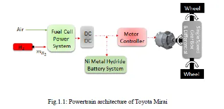
A Toyota Mirai power train architecture is as presented in figure 1.1, the vehicle is powered via an electrical traction system comprising of AC induction motors and motor controllers. The mechanical output from the electric traction motors is summed up in a single-speed summation gearbox. A differential couples the output of the summation gearbox to the wheels (car rear wheels).

The electrical traction system is powered by DC energy from two sources:

1: A fuel cell power system that converts the stored chemical energy in the hydrogen to DC electrical energy. The DC/DC convertor post the fuel cell power system is used to supply the DC electrical energy at a fixed voltage (660V). The fuel cell power system is sized for providing the average energy while traversing a drive cycle or meeting sustainable top speed requirements on different road conditions (level, flyovers, Ghats etc.)

2: A 660V Nickel Metal Hydride battery module that caters to the instantaneous traction power requirements of the electrical tractions system beyond that of the fuel cell power system. To cater to absorbing the regeneration power as a fuel cell is incapable of absorbing any energy.

1.3. Literature Review

Fuel cell-powered hybrid vehicles have demonstrated as an alternative solution that could replace the current Internal Combustion Engine based propulsion system because of the depletion of the fossil fuels and associated emissions. Researchers worldwide have taken several research and development initiatives over the past two decades since Fuel cell-powered hybrid vehicles would decrease both the nation's dependence on fossil fuels and pollution to the environment. The fuel cell takes a significant role in Fuel cell-powered hybrid vehicles as an important component and subsystems, being a new kind of power source to complement or replace conventional ICE. The fuel cell has a history of over 160 years since Sir William Grove had first invented it in 1839.

Qiuli Yu et al [2] (2008) proposed a fuel cell system model, the dynamic behavior of a fuel cell power system can be simulated and analyzed, which enables one to design a fuel cell control system, Simulation result shows that both the flow rate and pressure regulators designed separately are able to adjust the fuel flow rate according to the current input, as well as maintain the ideal cathode pressure.

Dongmei Chen et al [3] (2004) modeled a membrane humidifier for automotive fuel cell systems and analyzed based on basic thermodynamic laws. They found that we can actively control the fuel cell inlet air by controlling the number of humidification cell units to maintain proper membrane humidification for the fuel cell stack.

David O.Kazmer[4](1997) proposed PEM technology of next-generation. He found that computer-integrated injection molding will control entire manufacturing facilities, enabling optimization of information and information flow design, production, maintenance, material handling, and inventory control.

Power Train Architecture

2.1 Mirai Power Train vs. Conventional IC Engine Power Train

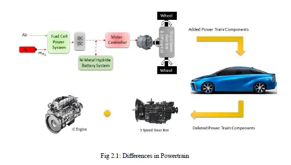
IC Engine and a gearbox found in conventional vehicles are replaced by fuel cell power train architecture to develop a fuel cell vehicle as shown in figure 2.1

A typical fuel cell power train consists of a fuel cell stack that powers the electric traction motors through its stack current along with the Nickel Metal hydride battery system which caters to the instantaneous traction power requirements of electrical tractions system which is beyond that of the fuel cell power system. The mechanical output from the electric traction motors is summed up in a single-speed summation gearbox. A differential couples the output of the summation gearbox to the wheels.

2.2 Overall Fuel Cell vehicle Power Train Architecture of a Toyota Mirai

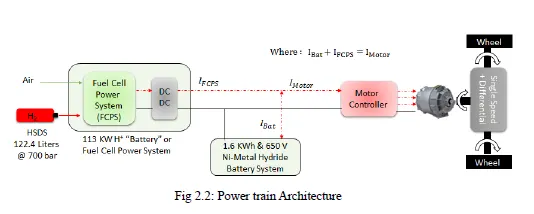
The overall fuel cell vehicle power train architecture of a Toyota Mirai is as presented in figure 2.2. The hydrogen H2 fuel required for the stack is provided through an onboard high pressure (700 Bar) H2 storage system. The fuel cell power system(FCPS) uses this onboard H2 to produce a stack current (IFCPS) which develops a maximum power of 113 KW that drives the traction motor system along with the 650 V Nickel Metal hydride battery which caters to instantaneous traction power requirement through the battery current (Ibat). Therefore the motor current (I Motor) is the summation of FCPS current (IFCPS) and the battery current (Ibat).

IMotor = IFCPS + IBattery…………………………………….... (2.1)

The mechanical output from the electric traction motors is summed up in a single-speed summation gearbox. A differential couples the output of the summation gearbox to the wheels.

2.3 Toyota Mirai Power Vehicle & Power Train Specifications

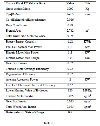
The following table provides the details regarding the inputs which are to be used in the model for arriving at the results, like the gross vehicle mass, the radius of the tire, its associated coefficient of rolling resistance, etc.

2.4 On-Board High-Pressure H2 Storage System

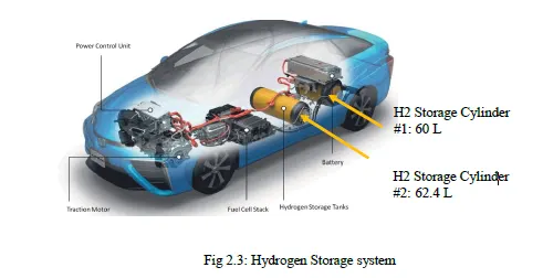
Figure 2.3 represents the onboard high-pressure H2 storage system of a Toyota Mirai. The system consists of two H2 cylinders of capacity 60L and 62.4L respectively.Hence the total onboard H2 storage capacity of the vehicle is 122.4L and the total weight of the system is about 85Kg. The H2 inside the cylinders is maintained at 700 Bar and 15 °C.

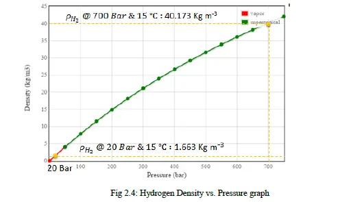
Figure 2.4 represents the variation of density (Kg/m3) of the H2 versus the H2 Pressure(Bar). It is noticeable that the density of H2 increases with an increase in H2 Pressure wherein H2 vapors forms into a supercritical state.H2 can be stored between 20 Bar to 700 Bar.

2.5: Force Analysis of Vehicle on an incline

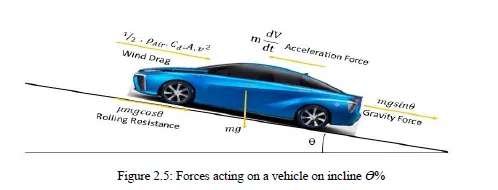
Let us consider a vehicle of mass m, moving with a velocity ν along a road gradient of Ө %. Due to the gradient, the vehicle's weight (mg) can be resolved into two components, mgSinӨ and mgCosӨ along the road gradient and normal to the road gradient respectively. This normal component mgCosӨ corresponds to a rolling resistance of μmgCosӨ where μ is the coefficient of friction. There also exists a drag force that opposes the motion of the vehicle. Therefore the force and power required at the wheels of the vehicle are given by:

Gravity Force: m.g.SinӨ………………………….…………………….... (2.2)
Rolling Resistance: μ.m.g.CosӨ……………………………………….. (2.3)
Acceleration Force: m.dv/dt…………………………………………….. (2.4)
Wind drag: ½ρACd ν2…………………………………………………….... (2.5)

Where: m = 2000 Kg
ρAir = 1.18 Kg/m ^3 ; Cd = 0.29
A=2.547 m2 Ө= 0%, for flyovers 4% and for ghat roads 7%

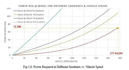
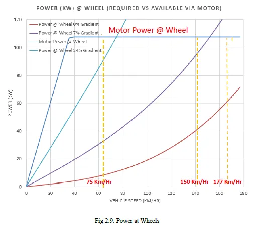
Figure 2.6 shows the plot of Power at wheel required versus vehicle speed for different gradients. At 0 percent gradient, 71 kW power is required at the wheel of the Toyota Mirai to move approximately 177 Km/hr. As the percentage gradient increases, the vehicle speed for the same power supplied decreases.

2.6: Electric Traction System & Governing Equations

Toyota Mirai is powered via an electrical traction system comprising of AC induction motors and motor controllers. The mechanical output from the electric traction motors is summed up in a single-speed summation gearbox. A differential couples the output of the summation gearbox to the wheels (car rear wheels). Hence selection of an Electric Traction System plays a vital role in vehicle performance.

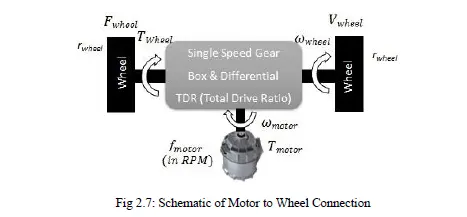
We know that vehicle speed is given by:
𝑉 = 𝑟 .𝜔 ………………….………................................. (2.6)

But,

𝜔wheel = 𝜔𝑀𝑜𝑡𝑜r/𝑇𝐷𝑅……………………………………………....... (2.7)

Where TDR= Total Driveline Ratio

𝜔 Motor=2𝜋𝑓Motor/60............................................. (2.8)

Therefore,
𝑉 = 𝑟𝑤ℎ𝑒𝑒𝑙 .2𝜋.𝑓𝑚𝑜𝑡𝑜𝑟/60.𝑇𝐷𝑅 ……..……………………………… (2.9)

The torque at the wheels can be represented as:

τWheel =Total Drive Ratio. 𝞰 Drive Line Losses. τMotor ( 𝟋 Motor) ………..……(2.10)
𝞰 Drive Line Losses = 98%
Ƭwheel =torque at the wheel
ƬMotor =torque at motor
𝞰 Drive Line Losses = Drive Line Losses efficiency
𝟋 Motor =speed of the motor

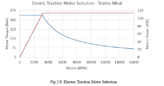
Figure 2.8 represents the plot of Motor Torque (Nm) and Motor Power (kW) versus the Motor RPM. At low Motor RPM, the motor torque is highest and it starts decreasing as the motor RPM increases above 3000 RPM. Similarly, as the Motor RPM increases, the Motor Power increases linearly and reaches saturation when the maximum rated power is reached. Therefore by selecting an appropriate Electric Traction System, required torque and vehicle speed can be obtained.

2.7: Electric Traction System Sizing Inference

Figure 2.9 below indicates the vehicle's top speed over different gradient % of roads along with the Power required and available at wheel. Though reserve power is available to reach speed in excess of 177Km/Hr on level roads.
However, the Traction Motor's peak RPM at 16000RPM and single-speed reduction ratio of 9.09 limits the top speed to ~177 Km/hr as justified below.

𝑉 𝑚𝑎𝑥=𝑟𝑤ℎ𝑒𝑒𝑙 .2𝜋.𝑓𝑚𝑜𝑡𝑜𝑟 𝑚𝑎𝑥/60.𝑇𝐷𝑅…………………... (2.11)

Substituting for the variable, we get

𝑉 𝑚𝑎𝑥=177 𝐾𝑚/ h𝑟

Fuel Economy Simulation

3.1. Toyota Mirai Fuel Economy Simulation Implementation

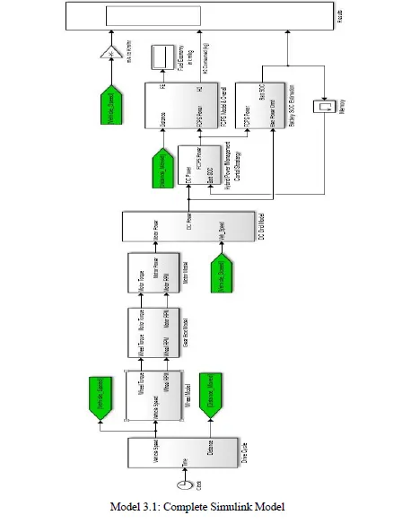
Model 3.1 is the Fuel Economy Implementation model, consisting of eight blocks which take a simulation time clock as the input, followed by a Drive Cycle model which takes in the time and giving us instantaneous vehicle speed and cumulative distance. These outputs from the first block is taken as input for the second block i.e. Wheel Model to get Wheel Torque and Wheel RPM. This output from the second block is taken as input from the second block into the third block i.e. Gear Box model wherein the Motor Torque and Motor RPM is calculated. Proceeding to the next block i.e. Motor Model the Motor Power required to run the motor to satisfy its power requirements. Then the net power required to run the Motor and the accessories in the vehicle after considering the power generated due to regeneration i.e. when the vehicle is decelerating is determined in the next model i.e. DC Grid Model. Using the DC Power and Battery State of charge as input to the next block i.e. Hybrid Power Management Control Strategy the net fuel cell power required i.e. the power required to be generated at the fuel cell power system is calculated. Going further the next block is FCPS Model which takes in fuel cell power required and distance and calculates the hydrogen consumed by the fuel cell to generate that much power and the fuel economy. There is a battery state of charge estimation model that estimates the battery state of charge using DC power and Electrical Power Demand as the input.

3.2: Drive Cycle Block

This block is used to determine the vehicle's instantaneous velocity and cumulative distance using the standard Drive Cycle. Standard data from the Environment Protection Agency website [1] is taken.For the simulation to be more realistic ,two data cycles wre the Urban Drive cycle at the start ,which represents urban/city driving conditions and the remaining part with a Highway drive cycle wthatrepresents highway driving conditions

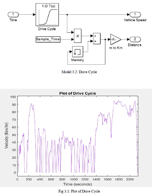
The plot in figure 3.1 is the Drive cycle i.e. plot of Vehicle velocity (in meters/second) vs. Time (in seconds), so for a given instant of time, velocity can be directly obtained from the plot. The instantaneous distance traveled can be obtained by multiplying it with the sample time. Therefore to calculate the overall distance traveled a memory block is used, wherein it stores the distance value and gives it back to the additional block in the next cycle. Summing up all the distances gives the cumulative distance. As the distance is in meters it is divided by 1000 to make it kilometer by including a gain block. Hence vehicle speed and cumulative distance are obtained from this block as output.

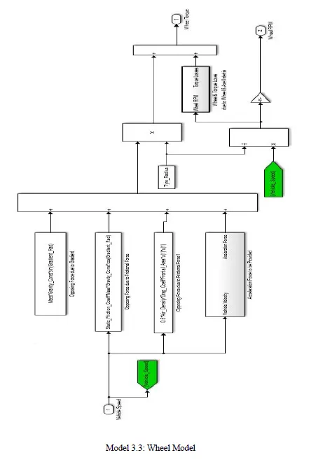
3.3: Wheel Model to calculate Wheel Torque and Wheel RPM

The Model 3.3 represents the block used to determine the instantaneous wheel RPM and instantaneous wheel torque required at the wheel. We know that,
Wheel Torque = Force * Tyre Radius ……………….……………………..…..................... (3.1)

Tire radius data is obtained from Table 2.1, the torque required is calculated and adding the torque losses due to wheel and axel inertia to obtain the net torque required
So,
Fwheel =Gravity Force+ Rolling Resistance + Acceleration Force +Wind Drag... (3.2)

Referring to the equations 2.1 thru 2.4 for Gravity Force, Rolling Resistance, Acceleration Force, Wind Drag we get,

Fwheel = mgSinӨ + μmgCosӨ+ m𝑑𝑣/𝑑𝑡 + 1/2 ρACd ν^2…………..……….…….….....(3.3)

Calculation of the acceleration force is shown in the following submodel (3.4)

3.3.1: Submodel A Acceleration Force to be provided

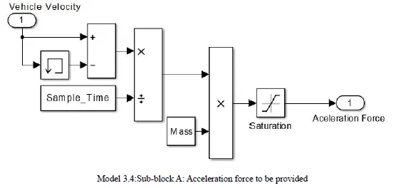
In Model 3.4, it takes in instantaneous velocity for that instant and subtracts it with the velocity of the previous instant given by the memory block,so you get the change in velocity after subtraction block i.e. dv and dividing it by sample time i.e. dt so to get dv/dt which is acceleration, multiplying it with the mass of the vehicle gives the force to be provided for the acceleration of the vehicle at that instant but only the force is needed while the vehicle is accelerating so a saturation block is added which only passes the value only if the force is positive or else it passes zero so which takes care of the situation wherein the force shouldn’t come in the picture while the vehicle is decelerating.

So the acceleration force is got from the sub-model 3.4, adding it according to the equation, total wheel force is obtained.

As we know,

Torque = Force * Radius……………..……………………. (3.4)

So multiplying the total force required at wheel by tire radius got from table 2.1, the torque required is determined. For the calculation to be more realistic and accurate, the Torque losses caused due to Wheel and Axel Inertia is added which is calculated as shown in the following submodel 3.3.2

3.3.2:Sub model B Wheel & Torque Losses due to Wheel & Axel Inertia

To make the model realistic and accurate the torque losses due to wheel and axel inertia are included which can be determined with the help of the sub-block B i.e. Wheel and Torque losses sub-block. Wherein the Torque losses can be calculated by the below equation.

𝑇=𝑑𝜔/𝑑𝑡……………………..…..……........................... (3.5)

Similarly, the instantaneous RPM can be determined with the help of the below equation,

𝑁=60𝑣/2𝜋𝑟….…………………………..………............…….. (3.6)

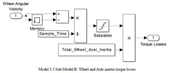
This sub-model takes in Wheel RPM, as there is memory block it gives the Wheel RPM to the subtraction block ahead with a delay to get dω, dividing it by sample time i.e. dt gives dω/dt which is angular acceleration α then it passed on through saturation element to get the positive values as the losses during deceleration cannot be negative and multiplying it with Total Wheel Axel Inertia in order to get Torque Losses.

Wheel Torque = Torque Required + Torque Losses…………………….. (3.7)

The total wheel torque to be supplied includes this torque required and the Torque losses caused due to Wheel and axel Inertia.
Now adding the Torque required with the torque losses got from the sub-model 3.5 Wheel Torque is obtained.
Taking Vehicle velocity and dividing it by tire radius got from Table 2.1, wheel angular velocity in radians/second is obtained. It is then multiplied by 60/2.π to convert it to RPM.
So, in this wheel model vehicle velocity is taken as input and after performing calculation according to the governing equations and some basic physics equation wheel torque and wheel RPM is obtained as output at the end of this model.

3.4 Gear Box Model

The instantaneous wheel torque and wheel RPM obtained from the Wheel Model is used to determine the instantaneous Motor torque and instantaneous Motor RPM using the Gear Box Model as shown above in model 3.6

The instantaneous Motor Torque required is a summation of Wheel Torque's product and the inverse of Total Drive Ratio and the Gear Box Torque losses due to Gear Box Inertia.

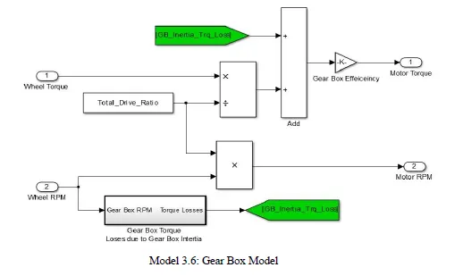
3.4.1: Sub Block to determine the Gear Box Torque Losses due to Gear Box Inertia

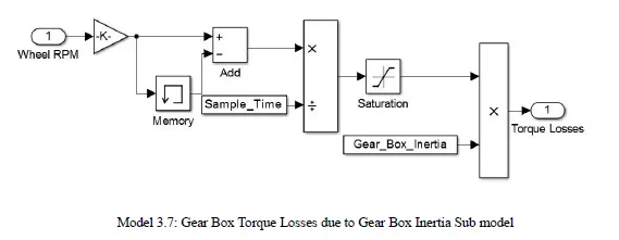
The Gear Box Torque Losses due to Gear Box Inertia is determined in a similar fashion as how the Wheel and torque losses due to wheel and axel inertia were found in the Wheel and torque losses sub-model.

This sub-model as shown in Model 3.7 takes in Gear Box RPM which is in runs per minute, to convert that angular velocity into radians per second it is multiplied by 2π/60 via gain block, proceeding further change in angular velocity is got by the combination of addition and memory block which is dω and dividing it by sample time i.e. dt gives us dω/dt i.e. nothing but 𝞪 which is angular acceleration. Angular acceleration can be positive or negative based on the velocity, as while deceleration i.e. negative angular acceleration there won’t be any fuel consumption we make the toque losses independent of it by adding a saturation block which passes the value only it is positive or else zero.Then multiplying angular acceleration by the Gear Box Inertia torque losses due to gearbox inertia is obtained.

3.5: Motor Model

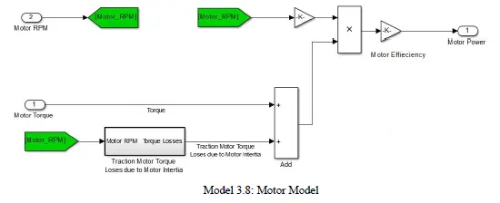
The instantaneous motor torque and instantaneous motor RPM which were determined using the Gear Box Model are used to determine the instantaneous Motor power required.

We know that,
Motor Power = Total Motor Torque * Motor Angular Velocity .……..……... (3.8)

But,
Total Motor Torque = Motor Torque + Torque losses due to Motor Inertia.… (3.9)

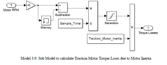
To find the torque losses due to motor inertia the sub-model 3.9 is used. Using the instantaneous Motor RPM as the input and the gain block is used to convert it to angular velocity due to the combination of memory and subtraction block, change in angular velocity which is dω is got and dividing it by sample time i.e. dt to get dω/dt which is 𝞪 i.e. Angular acceleration, as the loss has occurred only when it has positive values we include a saturation block for that purpose, which gives only positive values as it is and if it is negative value it gives zero. After which it is multiplied by Traction motor inertia to get the torque losses due to its motor inertia.
With reference to the equation, 3.9 torque losses are added and motor torque to get the net Torque required. The actual Motor Power required is obtained through the formula

𝑃=𝜂2𝜋𝑁𝑇/60………………………….……………………… (3.10)

Where,
P =Actual Motor Power required (W)
N= Instantaneous Motor RPM
T= Net Motor torque (Nm)
𝜂= Traction Motor Average Efficiency

So motor RPM multiplied by 2π/60 and with the Total Torque by using a multiplication block and then multiplied by the inverse of Traction Motor average Efficiency to get the Motor Power.

3.6: DC Grid Model

This block is used to determine the instantaneous power i.e. DC Power which needs to be generated by the fuel cell

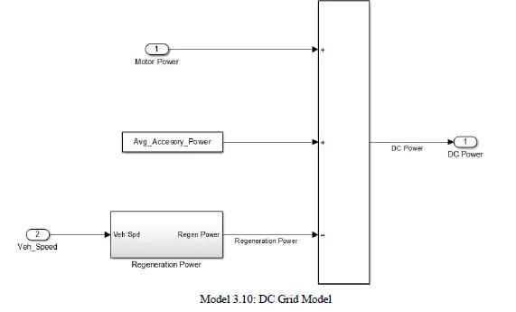
This block considers the motor power required along with power required to run the accessories and the power which is got by brake power regeneration to determine the net instantaneous power, i.e. DC Power, which needs to be generated the fuel cell.

3.6.1: Regeneration Power Sub Model

A regenerative brake is an energy recovery mechanism that slows a vehicle or object by converting its kinetic energy into a form that can be either used immediately or stored until needed in our case it is converted back to an electrical battery and stored in the Battery.

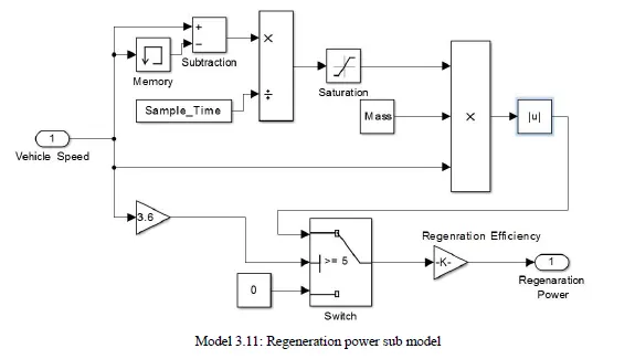
The above model shows a regeneration power block that determines how much power is regenerated while it is decelerating. Vehicle Speed is the input of this model wherein change in vehicle speed is determined by the combination of memory and subtraction block which gives us dv diving it the sample time i.e. dt gives us dv/dt which is acceleration, as the power is regenerated only when is the vehicle is decelerating the saturation block is added parameterizing it to only pass the negative values then multiplying it my mass gives the force then it passes thru Zero-Crossing Detection block to vary the time step size and enters the switch data port.

The switch has three input ports which are two data ports and a control port in the middle. If the predefined condition is met only then the data in port one (top one) is passed as the output or else the data in port three (bottom one) is passed as the output.

The purpose of using the switch block is to make sure that it calculates the power regenerated while the vehicle is decelerating until the vehicle speed reaches 5 km/hr which is the crawling speed of the vehicle because if the regeneration is still active below the crawling speed it would not stop as you want it to, it will have a long braking distance.

Then multiplying power with regeneration efficiency to obtain the actual power regenerated as there would be losses due to its mechanism.

3.7: Hybrid Power Management Control Strategy Model

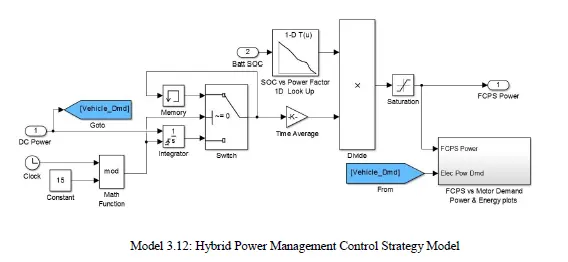
In order to understand the Hybrid Power Management Control Strategy Model, it becomes necessary to learn the basic idea behind the working of the model. The DC power required to drive the vehicle is to be supplied from the two sources i.e. Fuel Cell Power System and Battery. Wherein, the Fuel Cell Power System supplies the average power and any instantaneous power required will be compensated by the Battery. This method is adopted since it is not advisable to vary the FCPS power in accordance with the rapidly varying DC power as it adversely affects the life of the Fuel cell stack.
But determining the FCPS average power is not easy as the DC power varies rapidly and also the Battery SOC (State Of Charge) is to be maintained 50% to 70% of its total charge so that the life of the battery is extended. In order to tackle this, the average DC power consumed in an already occurred time interval is used to predict the average FCPS power to be maintained in the next time interval i.e. the average DC power consumed is determined for a certain time interval, using which the average FCPS power is predicted for the next time interval assuming that the similar pattern for DC power requirement continues.

Now coming back to the model, the total DC power is calculated for each time interval (say 15sec) and the new total DC power calculated gets updated, once the previous time interval is completed. This new total power is divided by the time interval to obtain the average DC power, which multiplied by the power factor obtained from the Battery SOC gives the average FCPS Power to be maintained.

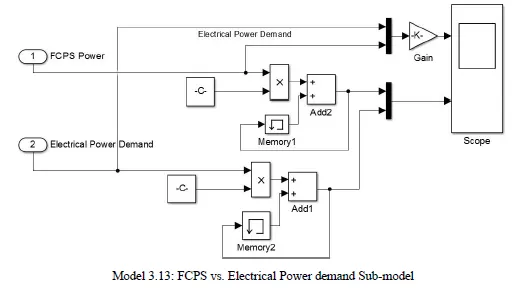
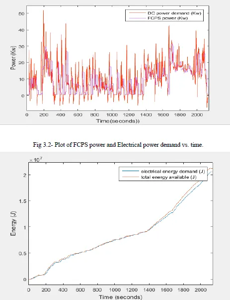
3.7.1: FCPS vs. Motor Demand Power and Energy plots Submodel

This sub-model as shown in Model 3.13 is used to obtain the plots of instantaneous FCPS power vs. instantaneous Electrical power demand and the total FCPS Energy vs. total Electrical energy demand. The instantaneous FCPS power and instantaneous Electrical power demand are obtained directly from the earlier model, whereas the instantaneous FCPS energy and instantaneous electrical energy demand are determined by multiplying the instantaneous FCPS power and instantaneous Electrical power demand with the sample time separately. Hence, the total FCPS Energy and the total Electrical energy demand can be obtained by adding their respective instantaneous energies using the memory block.

3.8. Battery State of the charge estimation model

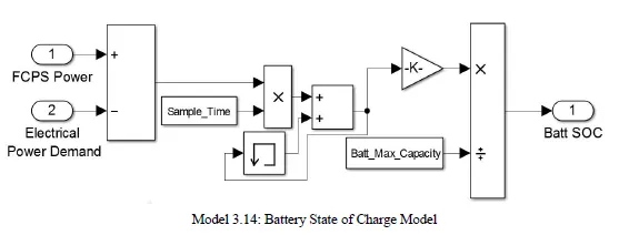
Battery State of charge is a parameter used to indicate the state of charge inside the battery i.e. how much electrical energy is there for use. Usually, for optimum performance of the battery, the State of charge is to be maintained between 50% 70%. Block 15 is used to estimate the Battery State of Charge as follows.The difference between the FCPS power and Electrical power demand gives the power supplied to the Battery. This power is used to determine the total energy of the battery. So the ratio of the battery's total energy and the maximum capacity of the battery gives the Battery State of charge.

3.9. FCPS model

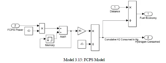
This block as shown in Model 3.15 is used to determine the Fuel Economy and the cumulative hydrogen consumed (Kg) from the FCPS power calculated using the Hybrid Power Management Control Strategy Model. The total FCPS energy is obtained from the FCPS power, using which the cumulative hydrogen consumed can be calculated by dividing the total FCPS energy by the lower calorific value of hydrogen. Hence, the ratio between the cumulative distance traveled and the cumulative hydrogen consumed gives the vehicle's Fuel economy.

Vehicle Performance simulation Implementation

4. Complete Simulation implementation for the vehicle performance

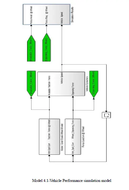
The model as shown in Model 4.1 is used to determine the vehicle's performance characteristics like vehicle speed, power available to the power required to drive the vehicle, and top speed. The simulation consists of four major models i.e. Motor, Gear Box and Wheel model; Force load on wheel model; Vehicle dynamics model and finally simulation results model. Each model will be discussed in detail in the subsequent sections.

4.1 Motor, Gear Box and Wheel model

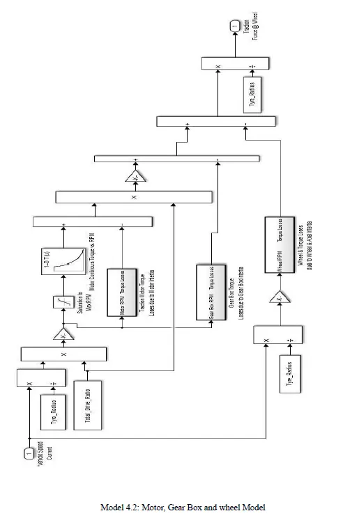
The Motor, Gear Box, and wheel Model uses the vehicle velocity to determine the wheel's traction force as shown in model 4.2. The vehicle velocity is divided by the wheel radius to obtain the wheels' angular velocity, multiplying it with the total drive ratio and suitable constant gives the motor RPM. Corresponding motor torque for the Motor RPM is obtained through the 1D lookup table.But there exist some torque losses due to motor inertia which is also taken into consideration for better accuracy.The net motor torque multiplied by the total drive ratio and total driveline losses gives the total wheel torque. There also exists losses due to gearbox inertia and the wheel axel inertia which are deducted from the total wheel torque to obtain the net torque at the wheels, which divided by wheel radius gives the Traction Force at the wheel.

4.1.1: Sub block to determine traction torque losses due to motor inertia

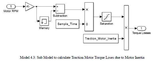
To find the torque losses due to motor inertia we use the sub-model 4.3. Using the instantaneous Motor RPM, which is the input and the gain block is used to convert it to angular velocity due to the combination of memory and subtraction block to get change in angular velocity which is dω and dividing it by sample time i.e. dt to obtain dω/dt which is 𝞪 i.e. Angular acceleration, as the loss has occurred only when it has positive values so a saturation block is included for that purpose, which gives only positive values as it is and if it is negative value it gives zero. After which it is multiplied by Traction motor inertia to get the torque losses due to its motor inertia.

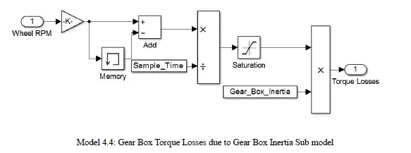
4.1.2: Sub Block to determine the Gear Box Torque Losses due to Gear Box Inertia

The Gear Box Torque Losses due to Gear Box Inertia is determined in a similar fashion as how motor inertia's motor losses were found in the Motor torque losses sub-model.
This sub-model as shown in Model 4.4 takes in Gear Box RPM which is in runs per minute, to convert that angular velocity into radians per second it is multiplied by 2π/60 via gain block, proceeding further to get change in angular velocity by the combination of addition and memory block which is dω and dividing it by sample time i.e. dt gives us dω/dt i.e. nothing but 𝞪 which is angular acceleration. Angular acceleration can be positive or negative based on the velocity, as while deceleration i.e. negative angular acceleration there won’t be any fuel consumption we make the toque losses independent of it by adding a saturation block which passes the value only it is positive or else zero. Then multiplying angular acceleration by the Gear Box Inertia we get torque losses due to gearbox inertia.

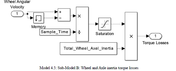
4.1.3:Sub model Wheel & Torque Losses due to Wheel & Axel Inertia

This sub-model in Model 4.5 takes in Wheel RPM, as there is memory block it gives the Wheel RPM to the subtraction block ahead with a delay to get dω dividing it by sample time i.e. dt gives dω/dt which is angular acceleration α then it passed on through saturation element to get the positive values as we don’t consider the losses during deceleration which does not account for any fuel consumption and it is multiplied by Total Wheel Axel Inertia gives Torque Losses at the end.

4.2: Force load on wheel model

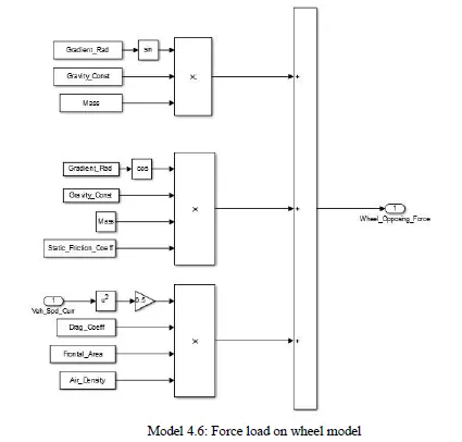
Model 4.6 is used to determine the opposing force acting on the wheels. We know that the force acting on a vehicle moving with a certain velocity is given by equation 3.3:

Fwheel = mgSinӨ + μmgCosӨ+ 0.5*ρACd u^2…………………………... (4.1)

Each term in equation 4.2 is mathematically modeled separately and added to obtain the total opposing force at the wheel as shown in Model 4.2.

4.3 Vehicle dynamics model

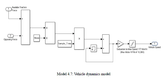
The available traction force and the opposing force determined from the previous model are subtracted to determine the acceleration's net force. So, dividing the net force available by vehicle mass gives the vehicle acceleration. Therefore the vehicle instantaneous velocity can be generated by multiplying the vehicle acceleration by sample time. Using the memory block the speed of the vehicle can be found. To make the model more realistic, the wheel slip is also considered while determining the vehicle's speed. However, the vehicle's maximum speed is limited to 177Km/hr as shown in equation 2.11.

4.4 Simulation results

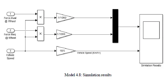
This model is used to generate the simulation results plot of vehicle speed, Power available vs. Power required at the wheel. The vehicle speed is obtained directly from the vehicle dynamics model, whereas the available power and required power are determined by multiplying vehicle velocity with the available force and required force respectively.

Results

5.1 Results for Fuel efficiency simulation implementation

5.1.1: Fuel Economy

After simulating the model a fuel economy of 85.73 km/kg i.e. it the vehicle can travel 85.73 km per kg of hydrogen was obtained.

5.1.2: Hydrogen Consumed

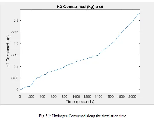
The above graph gives an idea of how hydrogen is being consumed by the Fuel Cell power system over the drive cycle simulation. Hydrogen consumed on the y-axis and time on the x-axis. We can notice that our averaging mechanism is working perfectly because the hydrogen consumption is steadily increasing along with time and not abruptly changing as the drive changes

5.1.3: Battery State of Charge:

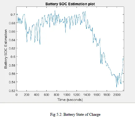
The Battery State of Charge graph above in Fig.5.2 gives us an idea of how the battery state of charge varies along with the simulation. As it is noticed from the graph that the battery state of charge is varying abruptly we can conclude that Battery is satisfying the instantaneous power demands according to the drive cycle.

5.2. Results for Performance Simulation Implementation

5.2.1: Vehicle Speed plot

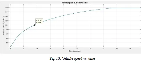
This plot gives the velocity of the vehicle at any given instant vs. time. Using the plot, the time the vehicle takes to accelerate from 0 to 100 Km/Hr is found to be around 9.145 seconds.

5.2.2: Plot of power available vs. power required at the wheel

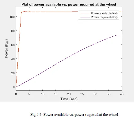
The above plot shows the Power required in blue color and the power available in red. We can infer from the plot that the power available is always greater than the power required so that the vehicle doesn’t fall short of the power required.

Conclusions and Future scope

6.1: Conclusions

The Modelling has been done and simulated in Simulink and we have got the results from Simulink. The Fuel Economy of the vehicle found using our simulation is approximately equal to the manufacturer specification, the error has crept in due to the assumptions made. The performance characteristic i.e. 0 100 km/hr and Maximum Vehicle speed, is well according to Manufacturer Data.

6.2: Future Scope

This type of vehicle modeling and simulation can be carried out for new generation vehicles with new technology, as the technology is still growing to make a prototype using that, testing it and then making some changes if it does not meet the requirements is very laborious time consuming and not cost-effective.Hence this would be an ideal solution for saving time and money.

References

[1]Drive Cycle data has been taken from the following website: http://www3.epa.gov/nvfel/testing/dynamometer.htm#vehcycles
[2]Qiuli Yu, Song Yul Choe, Anurag K.S (2008)improved modeling and control of a PEM Fuel Cell Power System for vehicles, A journal on fuel cell power systems
[3]Dongmei Chen and Huei Pengl,(2004) Modelling and simulation of the PEM Fuel cell Humidification System ,Proceeding of 2004 America Control Conference Boston ,Massachusetts
[4]David O.Kazmer (1997) Polymer injection molding technology, for next millennium, journal of injection molding technology