Modelling of Electric Rickshaw using Simulink
Electric Rikshaw:-
Electric rickshaws (also known as electric tuk-tuks or e-rickshaws or auto) have been becoming more popular in some cities since 2008 as an alternative to auto rickshaws and pulled rickshaws because of their low fuel cost, and less human effort compared to pulled rickshaws. They are being widely accepted as an alternative petrol/diesel/CNG auto rickshaws. They are wheelers pulled by an electric motor ranging from 650-1400 Watts. They are mostly manufactured in India & China, only a few other countries manufacture these vehicles.
The electric automobile did not easily develop into a viable means of transportation. Research waned from 1920-1960 until environmental issues of pollution and diminishing natural resources reawakened the need of a more environmentally friendly means of transportation. Technologies that support a reliable battery and the weight of the needed number of batteries elevated the price of making an electric vehicle.[7] In 1837, Robert Davidson of Scotland appears to have been the builder of the first electric car, but it wasn't until the 1890s that electric cars were manufactured and sold in Europe and America. During the late 1890s, United States roads were populated by more electric automobiles than those with internal combustion engines.
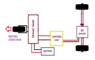
The Basic Electric Auto Rikshaw Power train Model:-
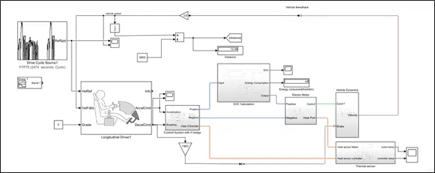
Simulink Model for Electric Rikshaw:-
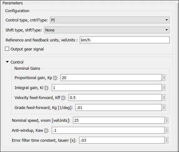
Longitudinal Driver:-
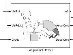
A parametric longitudinal speed tracking controller for generating normalized acceleration and braking commands based on reference and feedback velocities.
Whenever the feedback speed of vehicle is less than the reference speed, the acceleration command is provided to controller, but as well as this vehicle increase above the reference value, the braking command is generated.
Control System Block with H-bridge:-
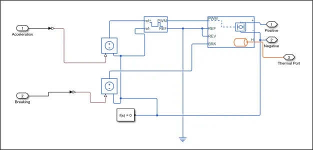
This sub-system consist of PWM converter, and H-bridge for the control of electric rikshaw.
Controlled PWM voltage:- This block creates a Pulse-Width Modulated (PWM) voltage across the PWM and REF ports. The output voltage is zero when the pulse is low, and is equal to the Output voltage amplitude parameter when high. Duty cycle is set by the input value. At time zero, the pulse is initialized as high unless the duty cycle is set to zero or the Pulse delay time is greater than zero.
H-bridge:- This block represents an H-bridge motor drive. The block can be driven by the Controlled PWM Voltage block in PWM or Averaged mode. In PWM mode, the motor is powered if the PWM port voltage is above the Enable threshold voltage. In Averaged mode, the PWM port voltage divided by the PWM signal amplitude parameter defines the ratio of the on-time to the PWM period. Using this ratio and assumptions about the load, the block applies an average voltage to the load that achieves the correct average load current. The Simulation mode parameter value must be the same for the Controlled PWM Voltage and H-Bridge blocks.
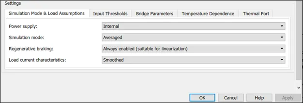
If the REV port voltage is greater than the Reverse threshold voltage, then the output voltage polarity is reversed. If the BRK port voltage is greater than the Braking threshold voltage, then the output terminals are short circuited via one bridge arm in series with the parallel combination of a second bridge arm and a freewheeling diode. Voltages at ports PWM, REV and BRK are defined relative to the REF port.
Electric System:- This subsystem contains the electrical components like, electric motor, which converts the electrical energy to the mechanical one.
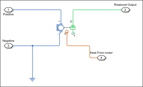
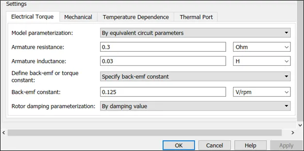
DC motor:- This block represents the electrical and torque characteristics of a DC motor. The block assumes that no electromagnetic energy is lost, and hence the back-emf and torque constants have the same numerical value when in SI units. Motor parameters can either be specified directly, or derived from no-load speed and stall torque. If no information is available on armature inductance, this parameter can be set to some small non-zero value. When a positive current flows from the electrical + to - ports, a positive torque acts from the mechanical C to R ports. Motor torque direction can be changed by altering the sign of the back-emf or torque constants.
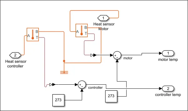
Thermal Sensor Sub-system:- In this sub-system we are calculating heat transfer from the motor and controller,
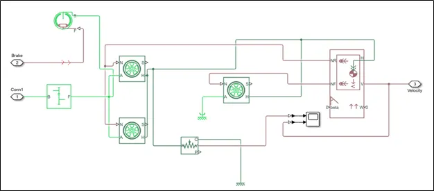
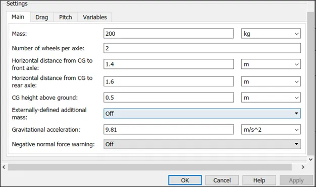
Vehicle Dynamics:- In this block, the actual vehicle parameters are define like tire, and chasis of vehicle, etc.
Tire:-

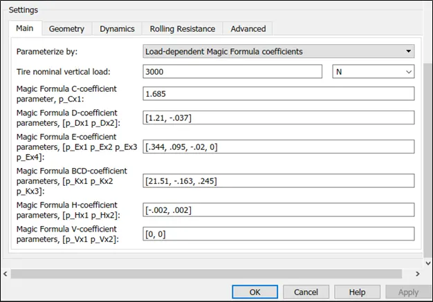
Represents the longitudinal behavior of a highway tire characterized by the tire Magic Formula. The block is built from Tire-Road Interaction (Magic Formula) and Simscape Foundation Library Wheel and Axle blocks. Optionally, the effects of tire inertia, stiffness, and damping can be included. Connection A is the mechanical rotational conserving port for the wheel axle. Connection H is the mechanical translational conserving port for the wheel hub through which the thrust developed by the tire is applied to the vehicle. Connection N is a physical signal input port that applies the normal force acting on the tire. The force is considered positive if it acts downwards. Connection S is a physical signal output port that reports the tire slip. Optionally expose physical signal port M by setting Parameterize by to Physical signal Magic Formula coefficients. Physical signal port M accepts a four element vector corresponding to the B, C, D, and E Magic Formula coefficients.
Vehicle Body:- This is graphical representation of vehicle body.
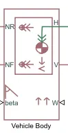
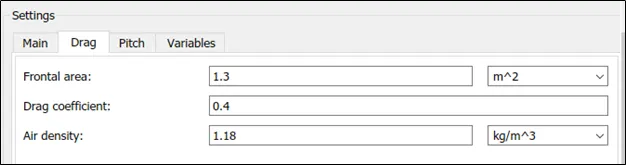
Represents a two-axle vehicle body in longitudinal motion. The block accounts for body mass, aerodynamic drag, road incline, and weight distribution between axles due to acceleration and road profile. The vehicle can have the same or a different number of wheels on each axle. Optionally include pitch and suspension dynamics or additional variable mass and inertia. The vehicle does not move vertically relative to the ground. Connection H is the mechanical translational conserving port associated with the horizontal motion of the vehicle body. The resulting traction motion developed by tires should be connected to this port. Connections V, NF, and NR are physical signal output ports for vehicle velocity and front and rear normal wheel forces, respectively. Wheel forces are considered positive if acting downwards. Connections W and beta are physical signal input ports corresponding to headwind speed and road inclination angle, respectively. If variable mass is modeled, the physical signal input ports CG and M are exposed. CG accepts a two- element vector representing the x and y distance offsets from vehicle CG to additional load mass CG. M represents the additional mass. If both variable mass and pitch dynamics are included, the physical signal port J accepts the inertia of the additional mass about its own CG.
Results:-
- Vehicle speed Vs Referance Speed.:- Here we are using FTP75 drive cycle for analysis.
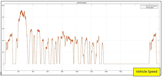
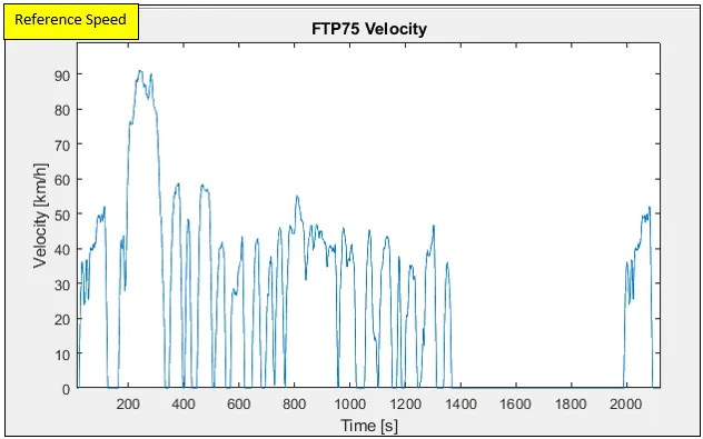
As we can see, both the curves are matching with each other.
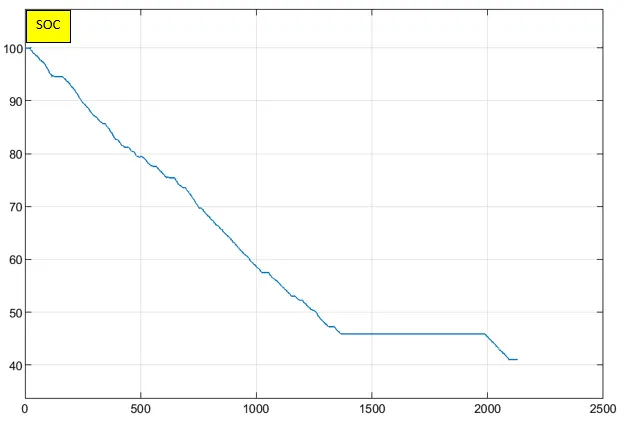
Below curves shows the SOC discharge of battery during simulation.
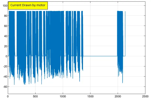
Also next graph shows the graph for current drawn by motor. As we can see current is continuously changing as the result of PWM signal input to motor.
Result for CUEDC drive cycle:-
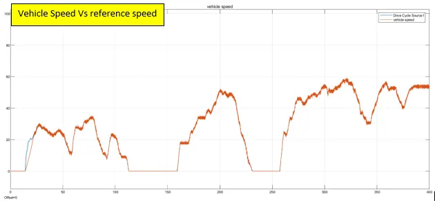
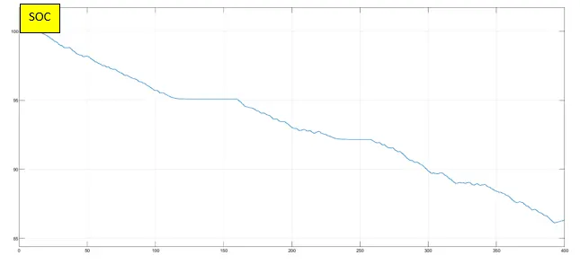
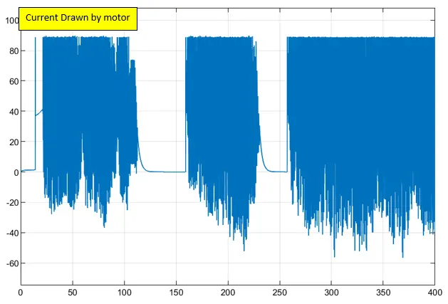
CUEDCs were created with the intention to closely replicate actual Australian on-road urban driving. CUEDCs are used for chassis based dynamometer testing of both heavy and light vehicles. They are composed of four distinct drive cycle segments: congested, minor roads, arterial and highway.
We can see for initial time when acceleration is high vehicle speed does not match the referance speed. The second figure shows SOC discharge.
Reference speed from Excel File:-
For this we experiment we created our own drive cycle. And provide this file as input to model as excel file.
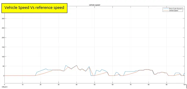
As we can see there is significant different between reference speed & vehicle speed when there is steep acceleration, for this we need to optimize our vehicle design, hence vehicle design is basically depend upon application, if we require very steep acceleration we need to have a motor which have very good response for variation in load.
Temperature increase in Motor and controller when Run at 45 Km/h for 100 sec.
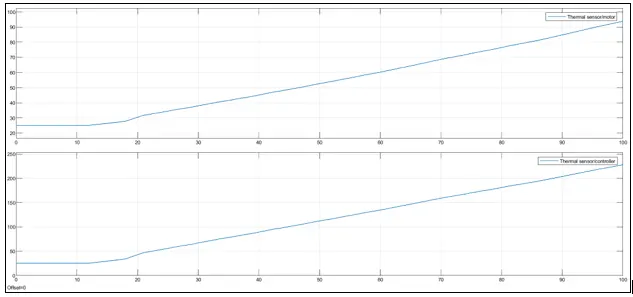
Motor temperature rise upto:- 80 C
Controller temp. rise upto:- 200 C
Conclusion:-
As per the Motor speciation, Type of controller, Vehicle Parameters & Battery used we could see that the reference speed almost matches with the vehicle for FTP75 drive cycle, but it not matched when we need a very steep acceleration. Hence we have to further change the parameters of the system and try simulating to achieve the results.
The Parameters that can be changed / Improved:
1) Optimization of Battery pack for increased mileage and peak performance
2) Optimization in the vehicle parameters such as vehicle mass, Front Area, Drag, Tire design etc
3) Better Motor characteristics or Motor such as BLDC motor, which reduces the losses produced from brushes and better efficiency. Hence Better motor power and Torque can be achieved
5) Use of actual PID Controller system rather than basic PWM signal generator block. This enables us to tune the system accordingly and brings down the error.
6)Provide better cooling arrangement to avoid losses.