Challenge

Mixing efficiency

DDipesh Salunke25 Aug 2020

Mixing Efficiency

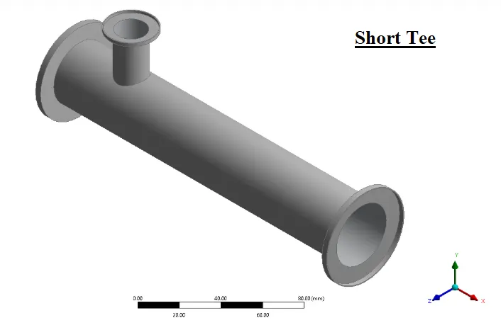
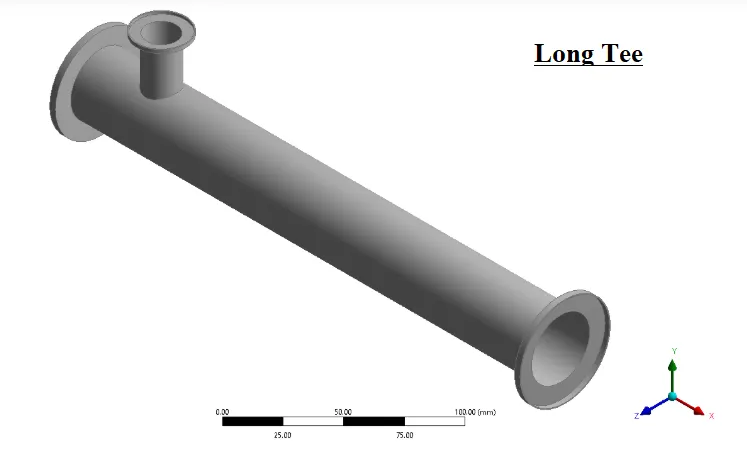
Two versions of the mixing tee is made using CAD software.One of them is longer than the other.

Steady-state simulation was set up to compare the mixing effectiveness when hot inlet temperature is 36⁰C & the Cold inlet is at 19⁰C.

Theory :

A Tee is formed by two pipe sections joined at a right angle to each other. The hot fluid (water) is flowing through the main pipewhile the cold fluid (water) enters the main pipe through the branched pipe. There have been traditionally developed empiricaldesign equations to solve the mixing problems but it does not take into account the complexity of turbulent flow in applications likepetrochemical products, waste water treatment, blending of oils, etc.

Nuclear industry is the one where efficiency of the mixing of fluids in the mixing chambers is very critical.

Standard k-e
The baseline two-transport-equation model solving for kinetic energy k and turbulent dissipation ε. Turbulent dissipation is the rate at which velocity fluctuations dissipate. This is the default k–ε model. Coefficients are empirically derived; valid for fully turbulent flows only.

Pros: Robust. Widely used despite the known limitations of the model. Easy to implement. Computationally cheap. Valid for fully turbulent flows only. Suitable for initial iterations, initial screening of alternative designs, and parametric studies.
Cons: Performs poorly for complex flows involving severe pressure gradient, separation, strong streamline curvature. Most disturbing weakness is lack of sensitivity to adverse pressure gradients.

Standard k-w
A two-transport-equation model solving for kinetic energy k and turbulent frequency ω. This is the default k–ω model. This model allows for a more accurate near wall treatment with an automatic switch from a wall function to a low-Reynolds number formulation based on grid spacing. Demonstrates superior performance for wall-bounded and low Reynolds number flows.

Pros: Superior performance for wall-bounded boundary layer, free shear, and low Reynolds number flows. Suitable for complex boundary layer flows under adverse pressure gradient and separation (external aerodynamics and turbomachinery). Can be used for transitional flows (though tends to predict early transition).
Cons: Separation is typically predicted to be excessive and early. Requires mesh resolution near the wall.

Mixing of the fluids inside the tee was simulated using ANSYS Fluent, a general purpose three dimensional CFD package. The turbulence model selected to setup the required case was k-ℇ.

Though Large Eddy Simulations (LES) and Direct Numerical Simulation (DNS) will give most accurate results in this case as it involves turbulent mixing, but many experiments have agreed to the fact that k-ℇ model reasonably agrees with the experimental results.As mentioned above, governing equations i.e. mass and momentum equations are solved using numerical methods as DNS wouldconsume a lot more computational power and time.

Mixing tee possess two inlets and one outlet. The momentum ratio for this type of tee is the ratio of velocity of cold fluid to velocity at mixed fluid at outlet.

(1) Case : 1

Short mixing tee with a hot inlet velocity of 3m/s.
Momentum ratio of 2, 4.

(2) Case : 2

Long mixing tee with a hot inlet velocity of 3m/s.
Momentum ratio of 2, 4.

Steps Involved in Simulation Setup :

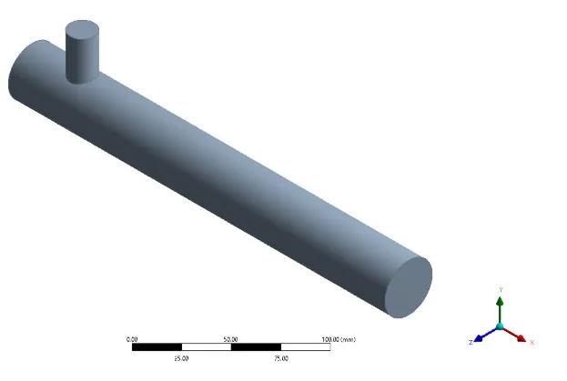
Creating the Flow Domain
Meshing of the Computational Domain
Setting up the Flow Physics & Solver settings
Post-Processing the Result

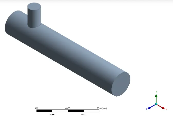
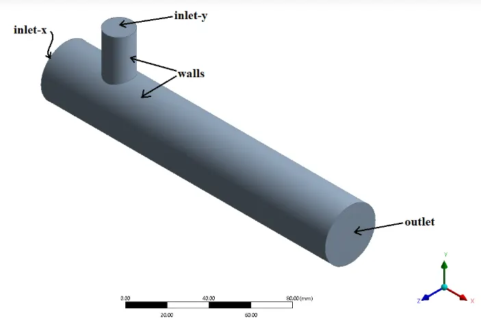
Case : 1(a) Short Tee with Momentum Ratio of 2

Grid Test :

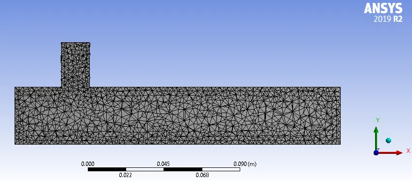
Mesh - 3mm

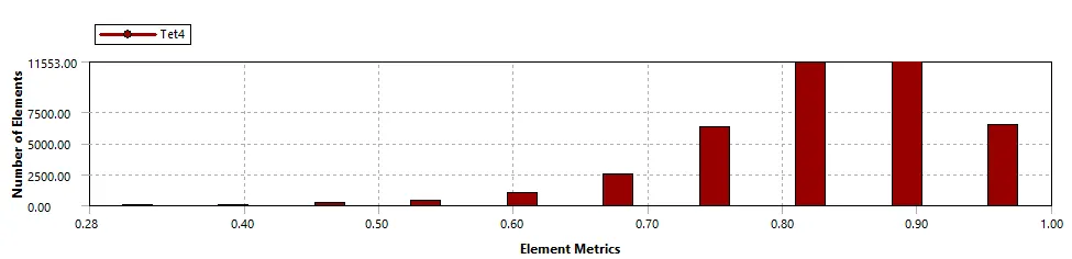
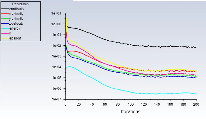
Residual Plot :

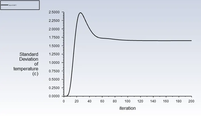
Standard Deviation of Temperature :

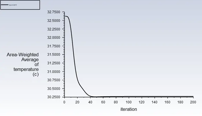
Area-Weighted Average of Temperature :

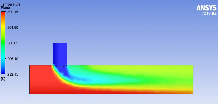
Temperature Distribution :

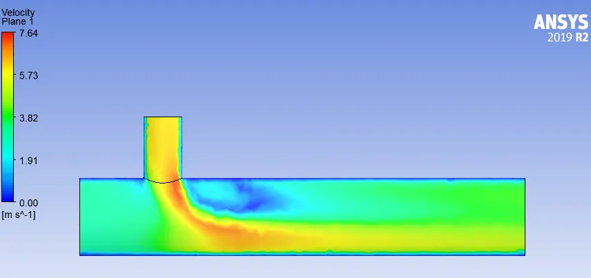
Velocity Distribution :

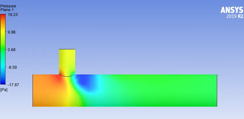
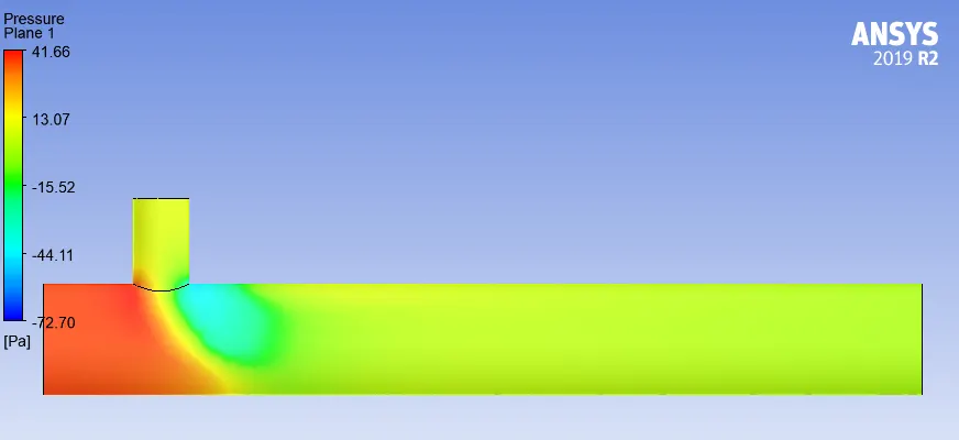
Pressure Distribution :

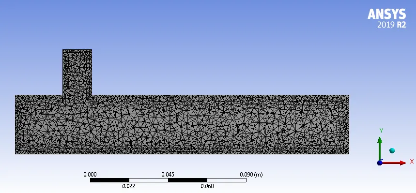
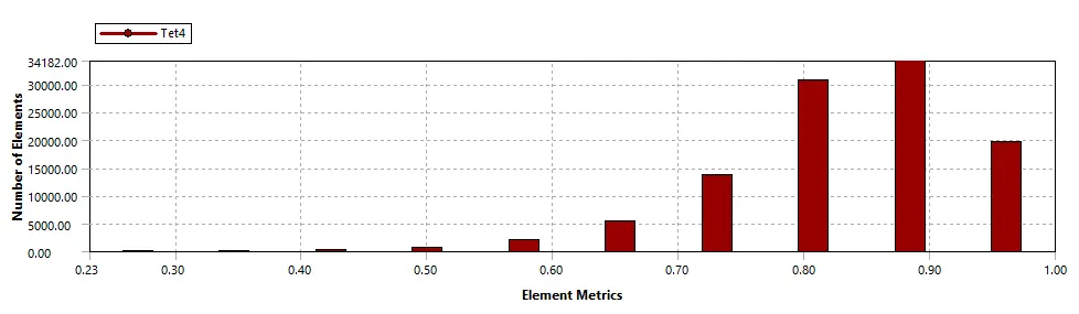
Mesh - 2mm

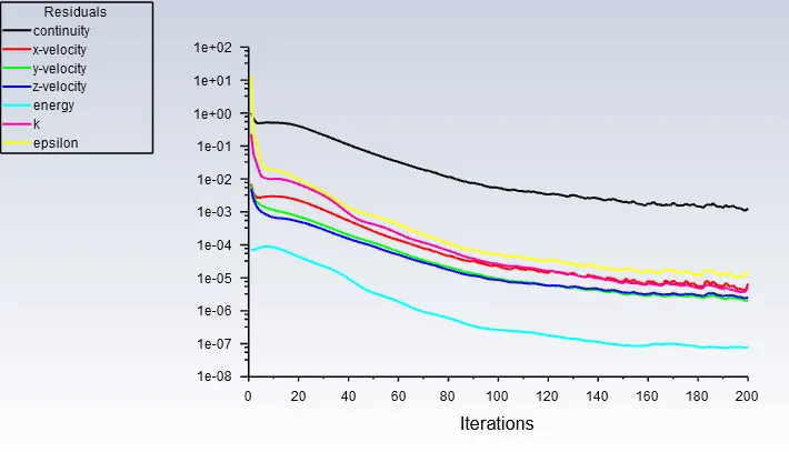
Residual Plot :

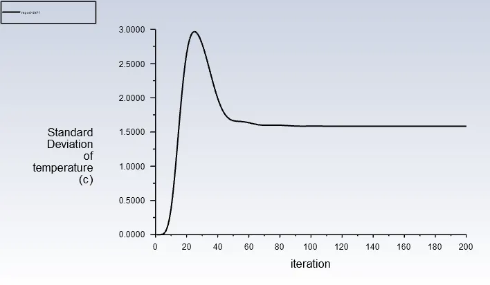
Standard Deviation of Temperature :

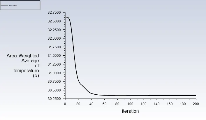
Area-Weighted Average of Temperature :

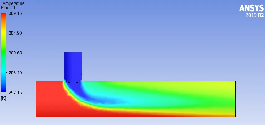
Temperature Distribution :

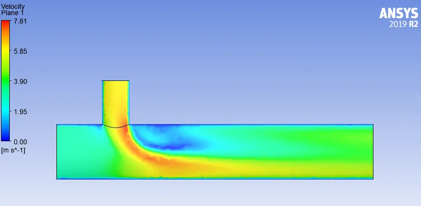
Velocity Distribution :

Pressure Distribution :

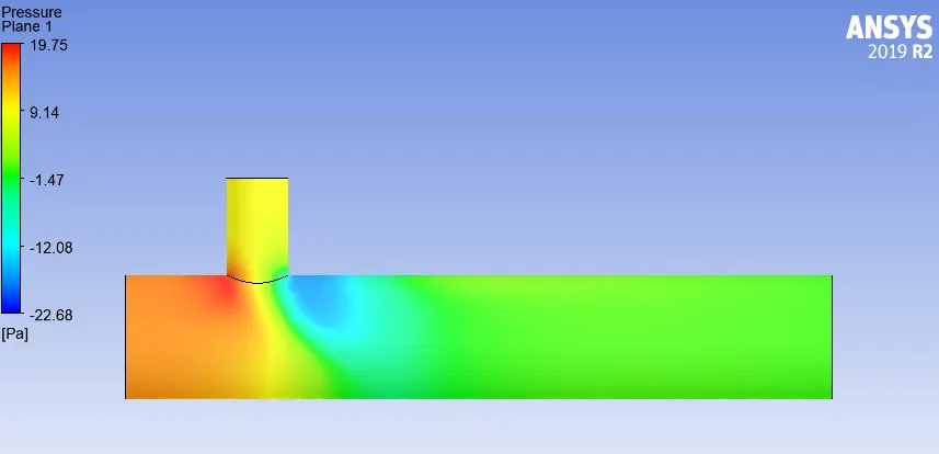
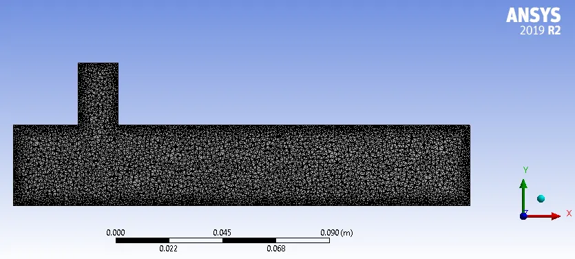
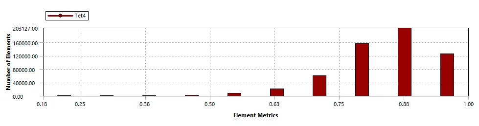
Mesh - 1mm

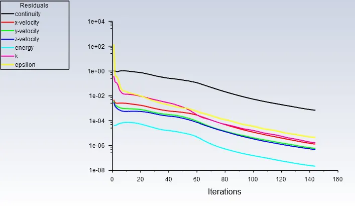
Residual Plot :

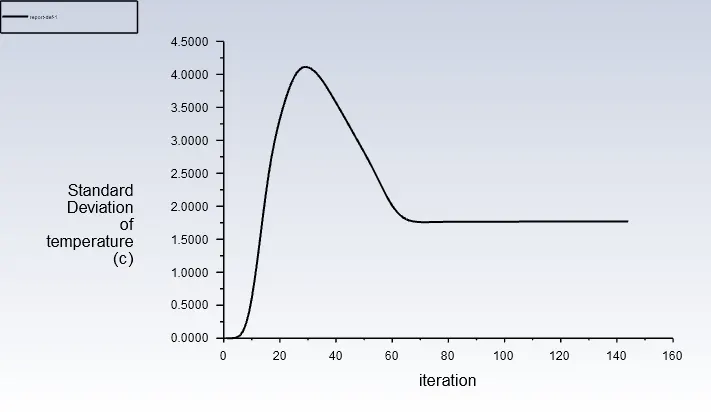
Standard Deviation of Temperature :

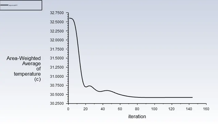
Area-Weighted Average of Temperature :

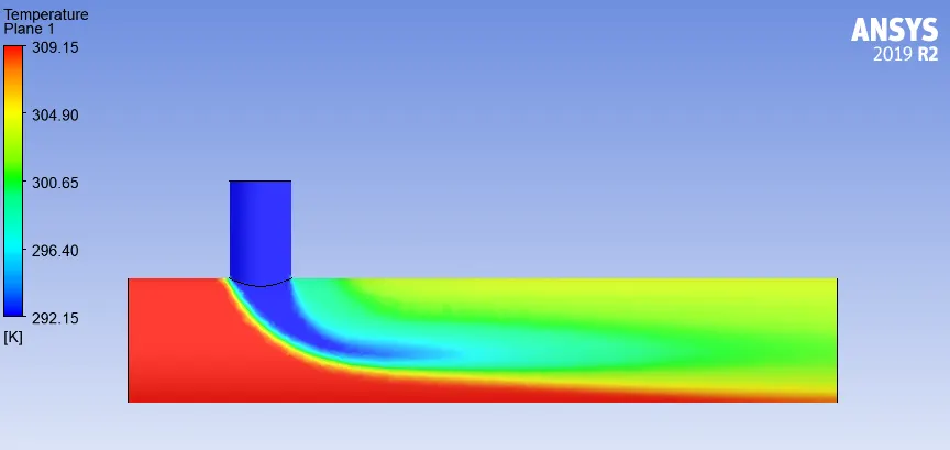
Temperature Distribution :

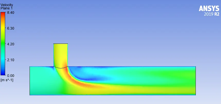
Velocity Distribution :

Pressure Distribution :

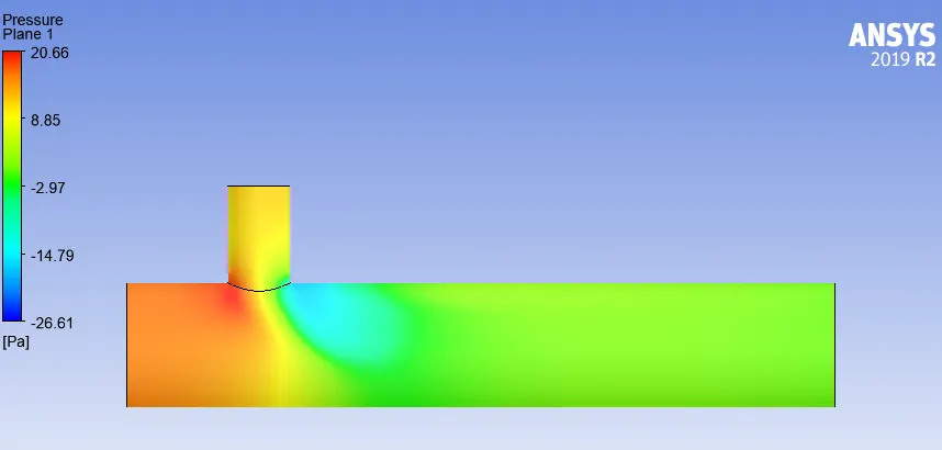
From the above grid dependence test, 2mm mesh size will be good choice for Academic License Package (Half Million Cells). It gives satisfactory results in this simulation.

So further, 2mm mesh will be used.

Case : 1(b) Short Tee with Momentum Ratio of 4

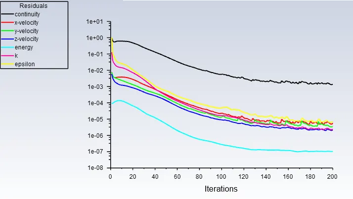
Residual Plot :

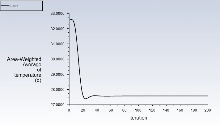
Area-Weighted Average of Temperature :

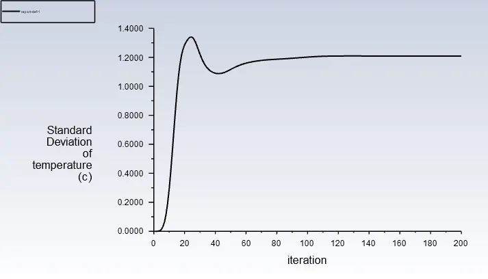
Standard Deviation of Temperature :

Temperature Distribution :

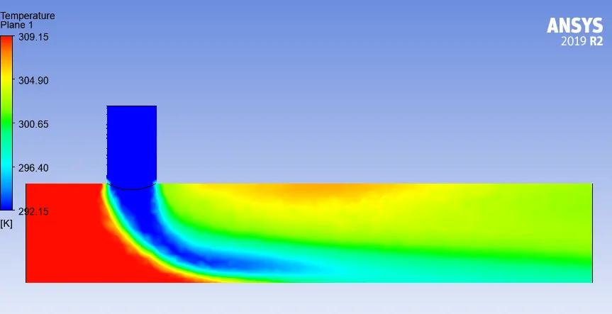
Velocity Distribution :

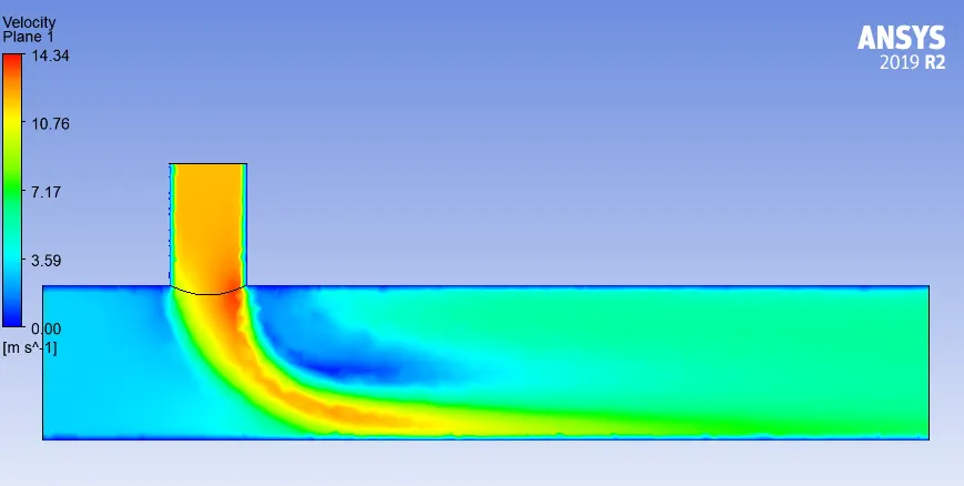
Pressure Distribution :

######################################################################

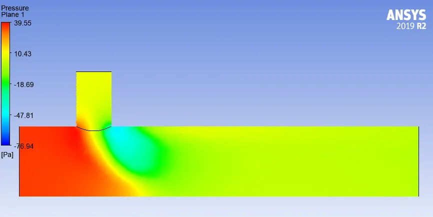
Case : 2(a) Long Tee with Momentum Ratio of 2

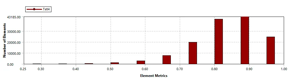
Mesh : 2mm

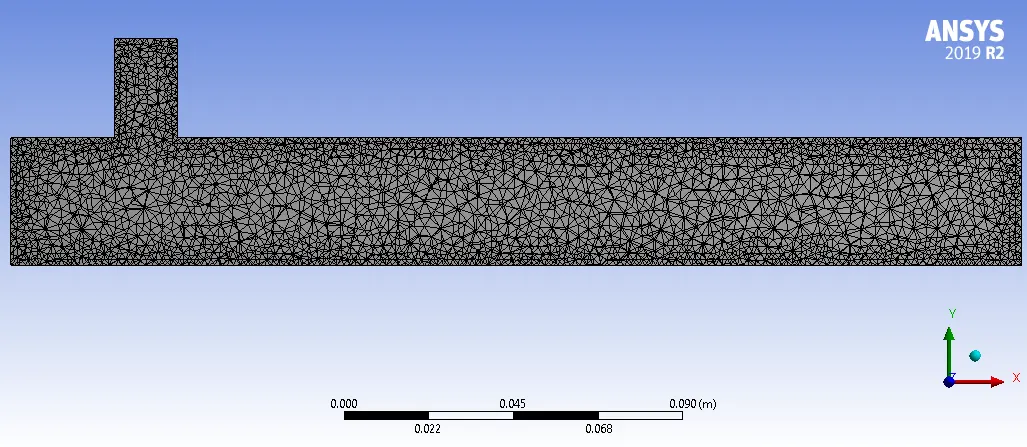
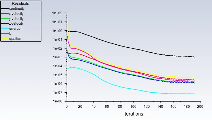
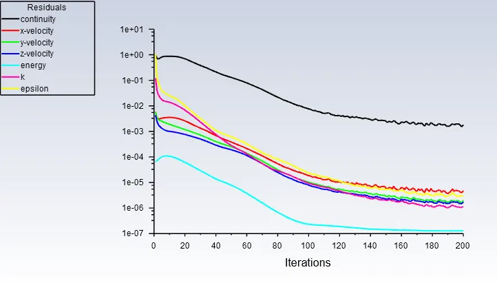
Residual Plot :

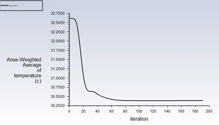
Area-Weighted Average of Temperature :

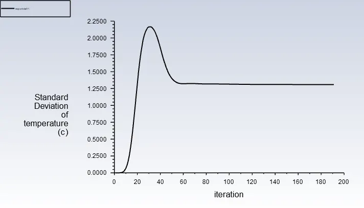
Standard Deviation of Temperature :

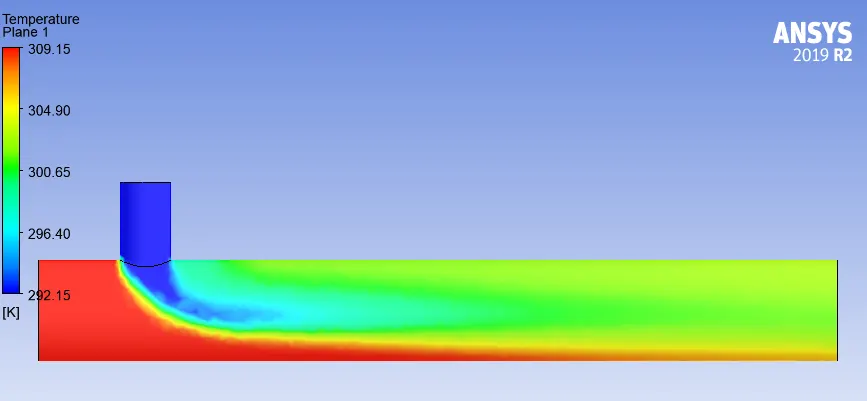
Temperature Distribution :

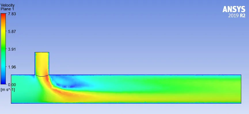
Velocity Distribution :

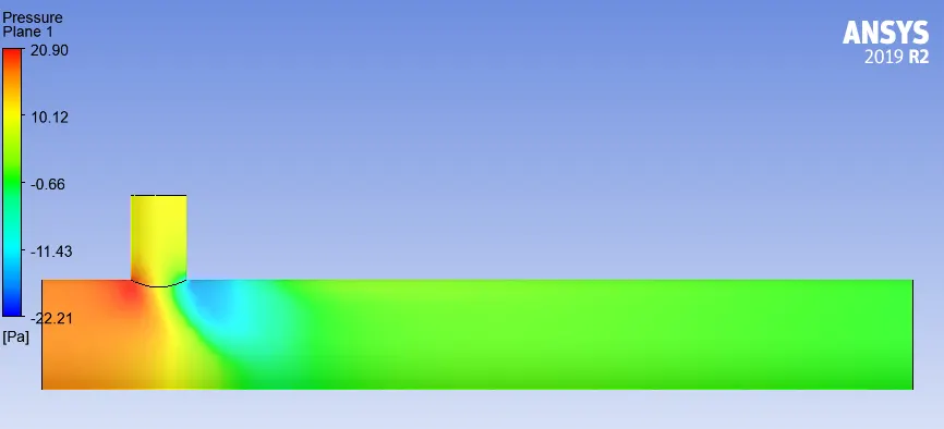
Pressure Distribution :

Case : 2(b) Long Tee with Momentum Ratio of 4

Residual Plot :

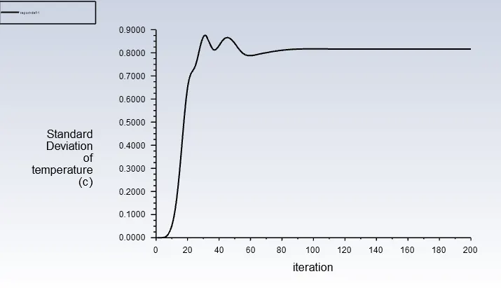
Standard Deviation of Temperature :

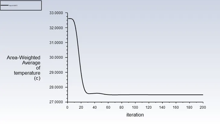
Area-Weighted Average of Temperature :

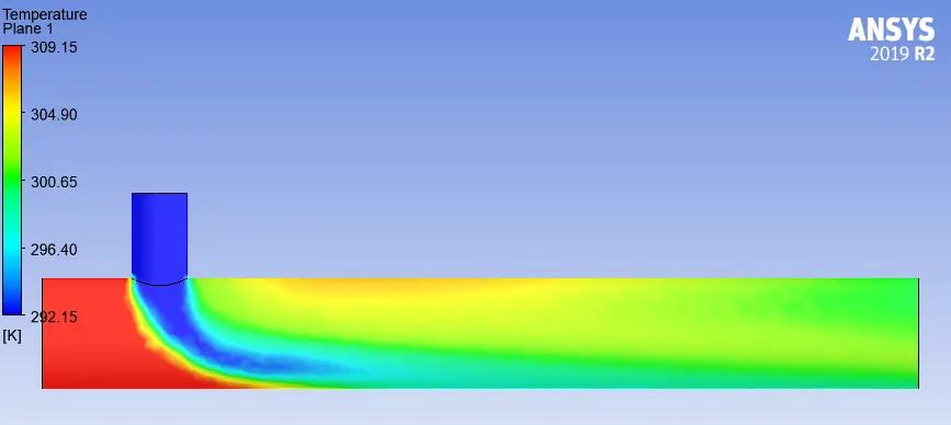
Temperature Distribution :

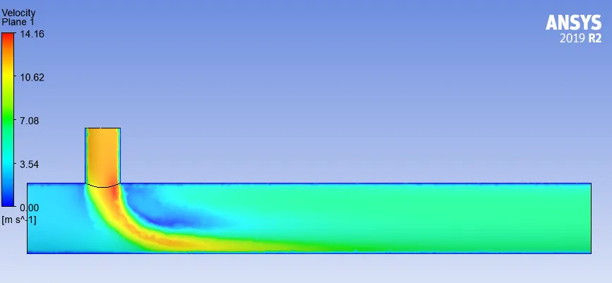
Velocity Distribution :

Pressure Distribution :

Conclusion :

From above table, we can see that Long Tee in both cases are not that much effective w.r.t. Short Tee. The Temperature & Velocity at outlet in case-2(Short Tee with Momentum Ratio-4) is satisfactory. It increase the material weight and cost only. So, mixing tee with momentum ratio 4 is good option because of better mixing efficiency.

Mixing efficiency

Ship work like this
in your own course.

Talk to a career counsellor

Ship work like thisin your own course.

Talk to a career counsellor

Ship work like this
in your own course.