Mixing efficiency

Aim: We have created two versions of the mixing tee. One of them is longer than the other.

Our job is to set up steady-state simulations to compare the mixing effectiveness when hot inlet temperature is 36⁰C & the Cold inlet is at 19⁰C.

Use the k-epsilon and k-omega SST model for the first case and based on your judgment use the more suitable model for further cases. Giving the reason for choosing a suitable model is compulsory.

Mixing Tee:

Fluid mixing is represented in the form of mixing two coaxial jet flows with good mixing efficiency. It is generally used for applications that require an efficient mix of two fluid streams with different physical & chemical properties combination together to form one stream. For example, this mixing Tee is used in high pressurised application like an Air Conditioner. In the mixing of Fluids, thus viscosity is a prevailing property of the system mixing if it is in lower the value the turbulent mixing can be achieved quickly and mixing operation can be easily done. Moreover, the standard deviation method used to examine the mixing efficiency in tee simulation.

1. Case 1
   • Short mixing tee with a hot inlet velocity of 3m/s.
   • Momentum ratio of 2, 4.

Momentum ratio = velocity at cold inlet / velocity at hot inlet.

*Short mixing tee with a hot inlet velocity of 3m/s and cold inlet velocity of 6 m/s using k-epsilon layer.

hot inlet temperature is 36⁰C & the Cold inlet is at 19⁰C.

K-epsilon layer:

This model is essentially a high Reynolds number model, meaning the law of the wall must be employed and provide velocity “boundary conditions” away from solid boundaries (what is termed “wall-functions”). Another major drawback is the model's lack of sensitivity to adverse pressure-gradient. It was observed that under such conditions it overestimates the shear stress and by that delays separation.

This model is usually used where flow does not demand to integrate the solution through the viscous sublayer and wall-bounded effects are secondary. For such cases, the first cell away from the wall shall be placed at a y+ of 30-300. In such a scenario, the viscous sublayer and buffer layer (viscosity-affected inner region) are not resolved. Instead, semi-empirical formulas called “wall functions” are used to bridge the viscosity-affected region between the wall and the fully-turbulent region.

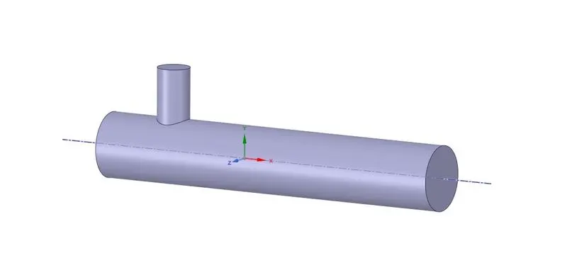
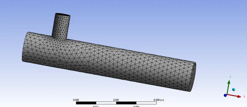
Geometry:

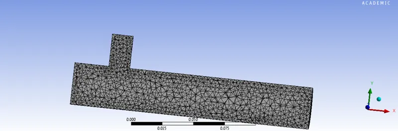
Mesh:

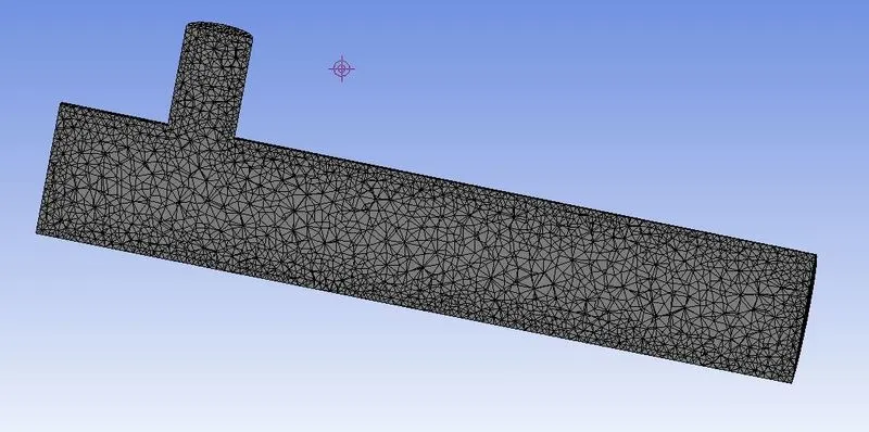
Cell count:

Element size:1.0219e-002m

Nodes:2797

Elements:12583

Element size:2e-003m

Nodes:21407

Elements:106253

Element size:1e-003

Nodes:110080

Elements:573275.

Here i have chosen mesh element size 2e-003m.

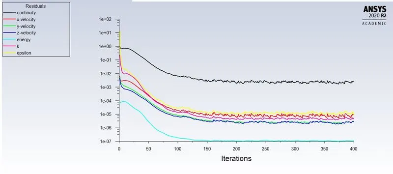
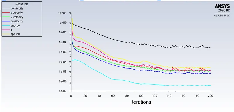
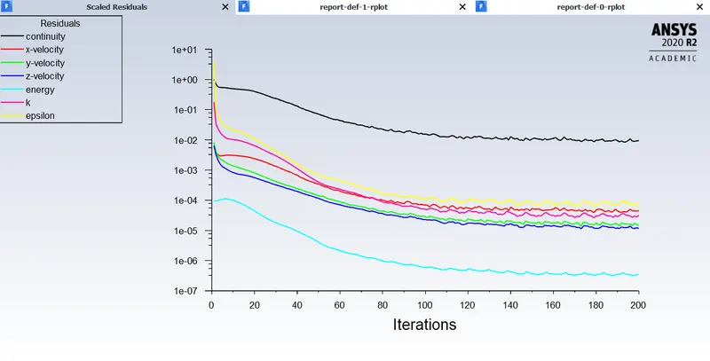
residuals:

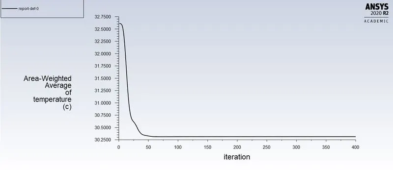
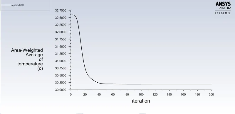
Average outlet temperature:

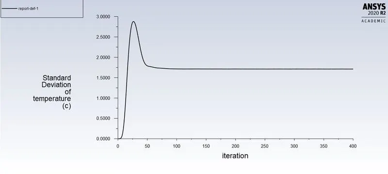
Standard deviation of temperature:

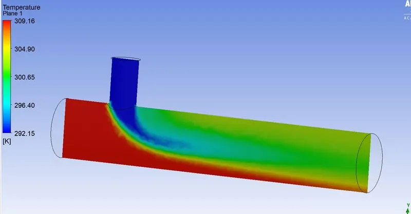
Temperature across the plane:

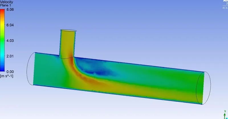
Velocity across the plane:

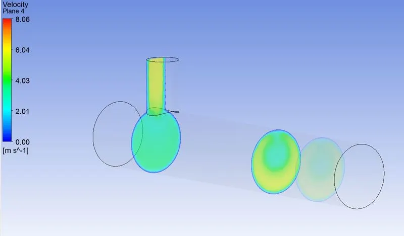
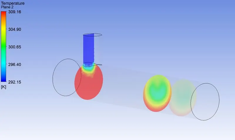
Velocity and temperature contour plots on the cut planes along and across the pipe:

Velocity:

Temperature:

Temperature line plot: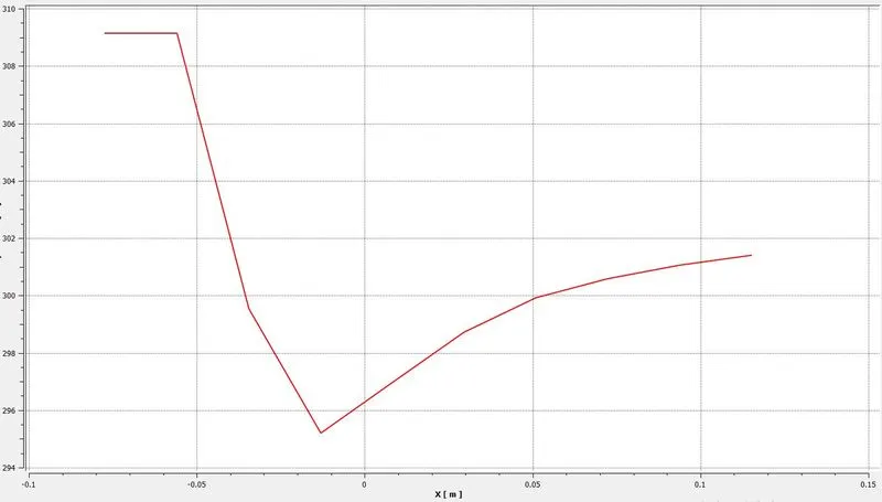

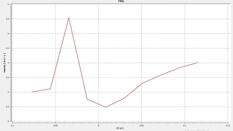
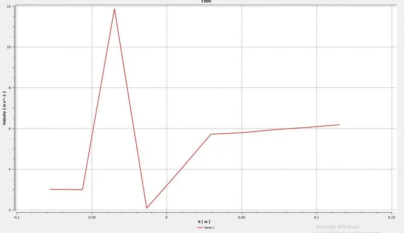
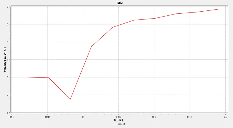
Velcoity line plot:

*Short mixing tee with a hot inlet velocity of 3m/s and cold inlet velocity of 12 m/s using k-epsilon layer.

when hot inlet temperature is 36⁰C & the Cold inlet is at 19⁰C.

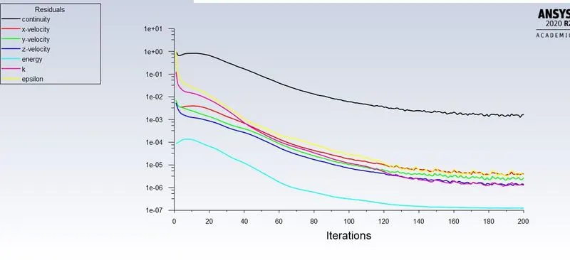
Residuals:

Average outlet temperature:

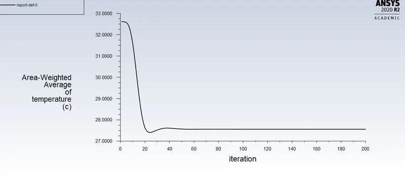
Standard outlet temperature:

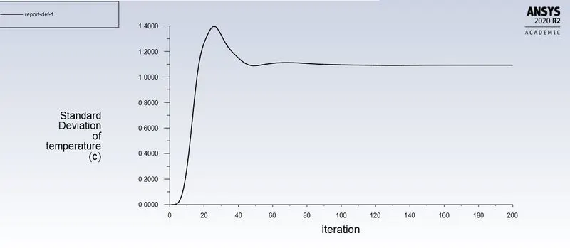
Temperature across the plane:

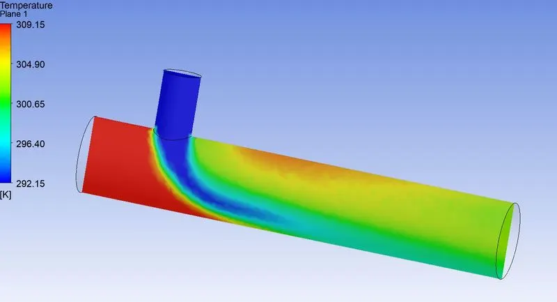
Velocity across the plane:

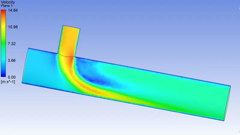
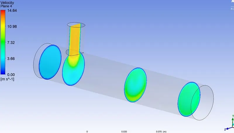
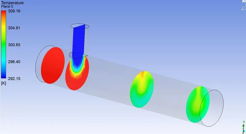
Velocity and temperature contour plots on the cut planes along and across the pipe:

Velocity:

Temperature:

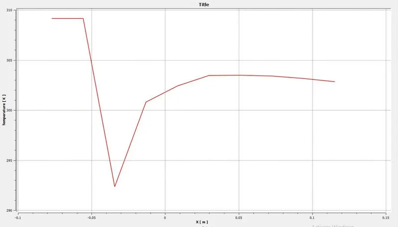
Temperature line plot:

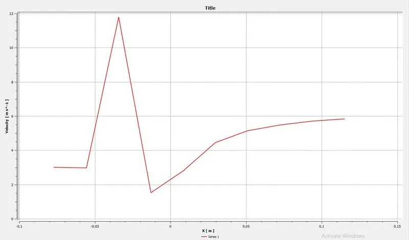
Velocity line plot:

*Short mixing tee with a hot inlet velocity of 3m/s and cold inlet velocity of 6 m/s using k-omega SST layer.

when hot inlet temperature is 36⁰C & the Cold inlet is at 19⁰C.

K-omega model:

This model is essentially a low Reynolds number model. This model takes 'elliptic' near-wall behavior meaning that it has an inherent nature of being able to “communicate” with the wall and actually has Dirichlet (as in no-slip in this case) boundary conditions. The implication of such behavior is the straightforward possibility of integrating through the laminar sublayer without additional numerically destabilizing damping functions or two additional transport equations.

Commonly encountered situations where the flow demands integrating through the viscous sublayer include: heat transfer, calculation of aerodynamic drag, flows with adverse pressure gradients, etc. Integrating through the viscous sublayer would generally impose resolving the mesh to y+<1. The omega equation can be integrated through the viscous sublayer without the need for a two-layer approach.

Residuals:

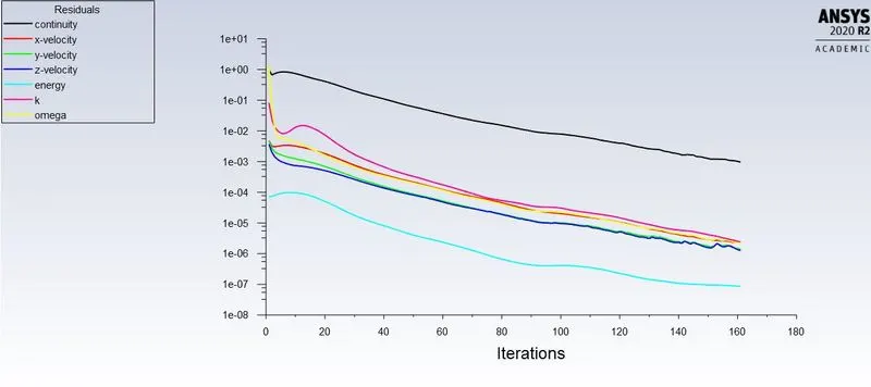
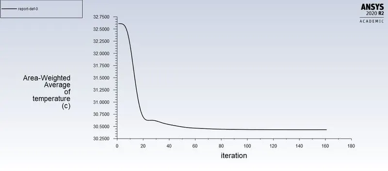
Average outlet temperature:

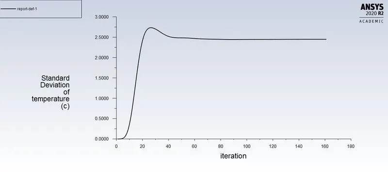
Standard deviation of the temperature:

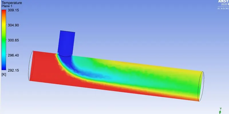
Temperature across the plane:

Velocity across the plane:

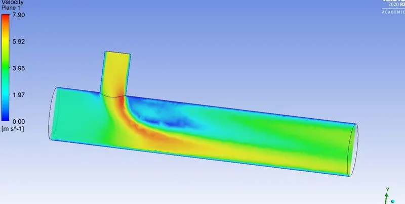
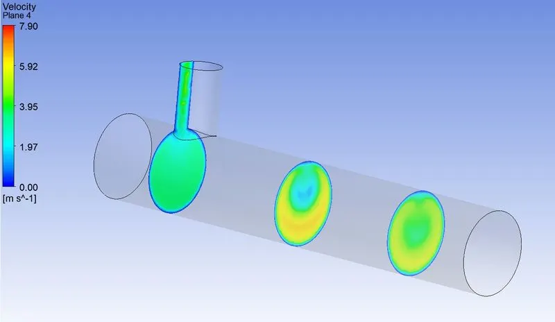
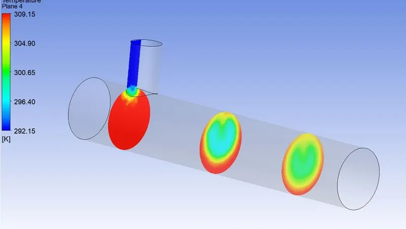
Velocity and temperature contour plots on the cut planes along and across the pipe:

Velocity:

Temperature:

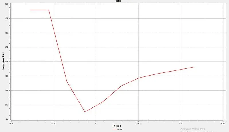
Temperature line plot:

Velocity line plot:

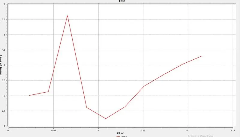
*Short mixing tee with a hot inlet velocity of 3m/s and cold inlet velocity of 12 m/s using k-omega SST layer.

when hot inlet temperature is 36⁰C & the Cold inlet is at 19⁰C.

Residuals:

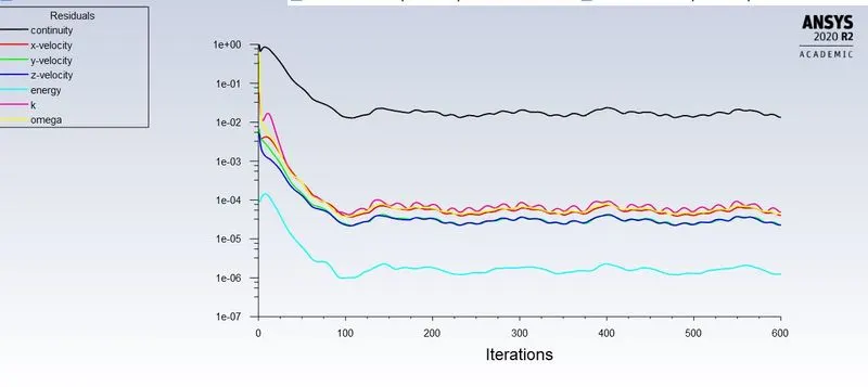
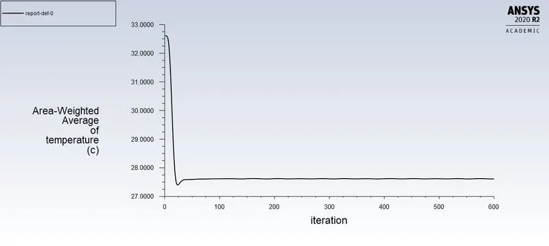
Average outlet temperature:

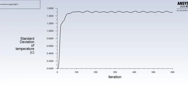
Standard deviation of temperature:

Temperature across the plane:

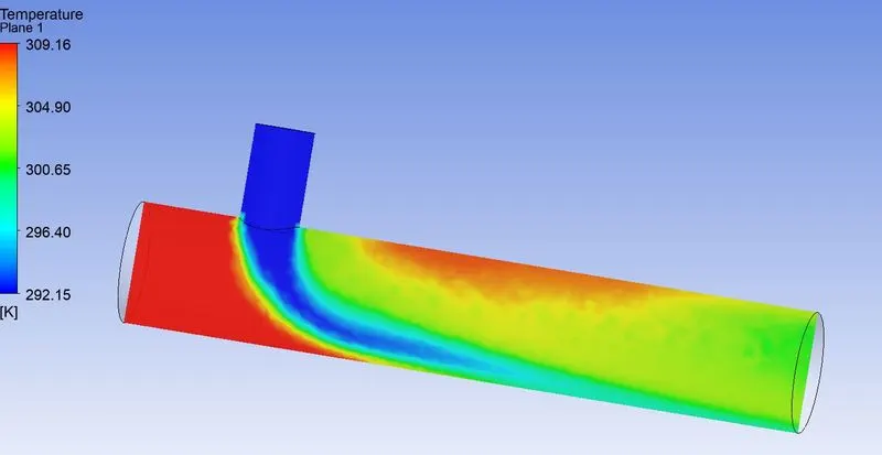
Velocity across the plane:

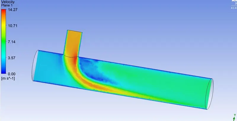
Velocity and temperature contour plots on the cut planes along and across the pipe:

Velocity:

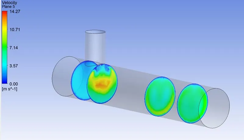
Temperature:

Temperature line plot:

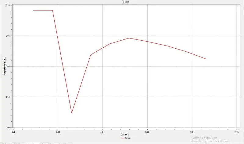
Velocity line plot:

Case 2

• Long mixing tee with a hot inlet velocity of 3m/s.
• Momentum ratio of 2, 4.

Momentum ratio = velocity at cold inlet / velocity at hot inlet

*Long mixing tee with a hot inlet velocity of 3m/s and cold inlet velocity of 6 m/s using k-epislon layer.

when hot inlet temperature is 36⁰C & the Cold inlet is at 19⁰C.

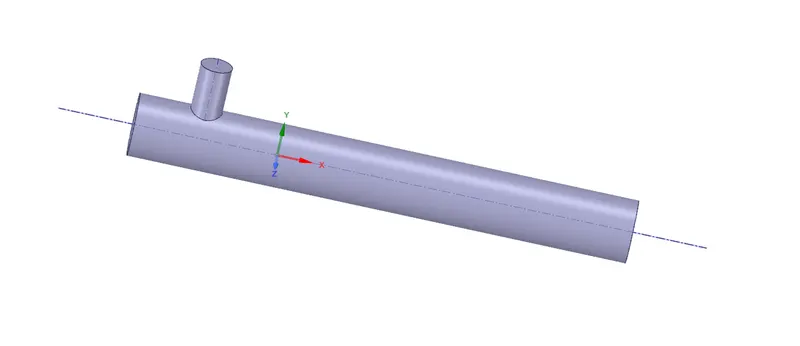
Geometry:

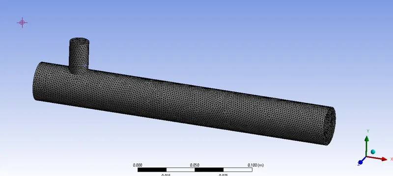
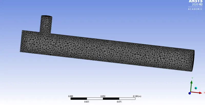
Meshing:

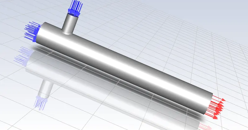
Cell count:

Element size:1.3853e-002m

Nodes:3432

Elements:15368

Element size:2e-003m

Nodes:28282

Elements:140025

Element size:1e-0003

Nodes:146441

Element:761659

Here i have taken element size 2e-003m.

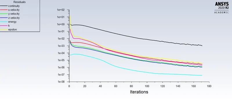
Residuals:

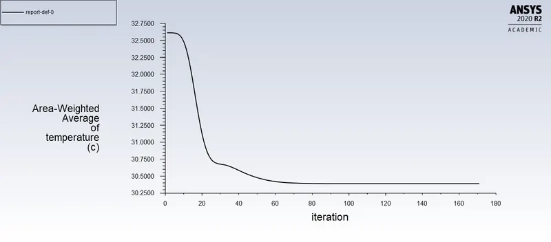
Average outlet temperature:

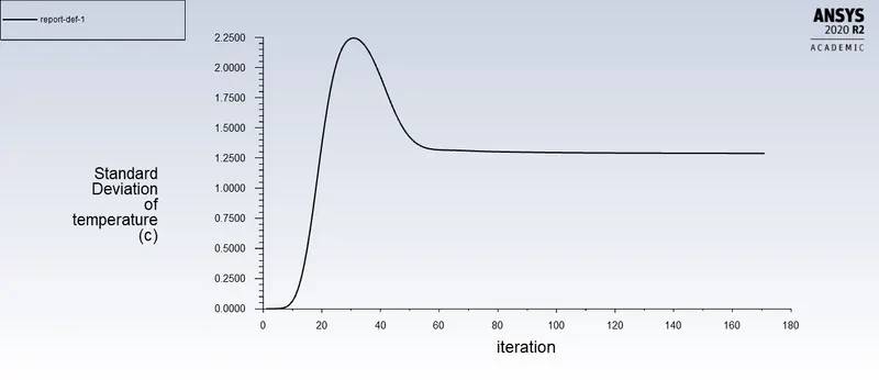
Standard deviation of temperature:

Temperature across the plane:

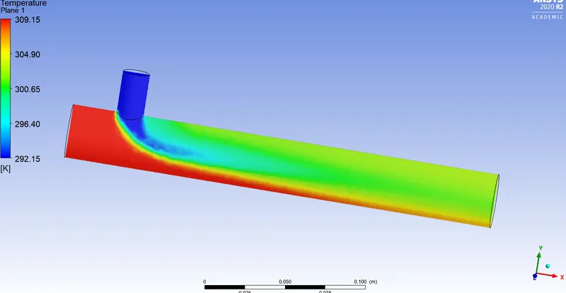
Velocity across the plane:

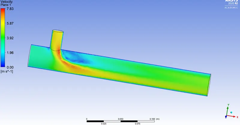
Velocity and temperature contour plots on the cut planes along and across the pipe:

Velocity:

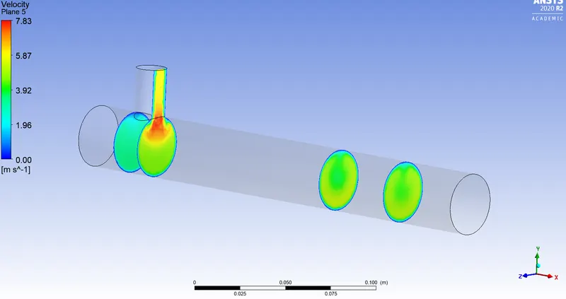
Temperature:

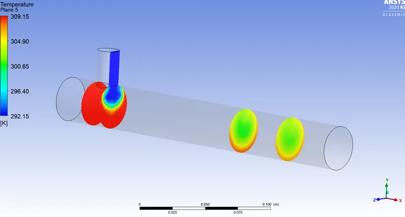
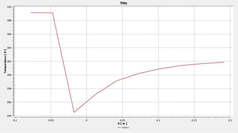
Temperature line plot:

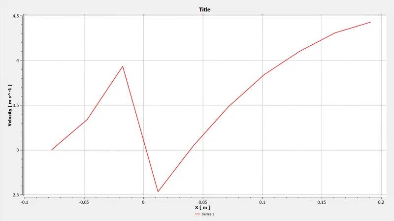
Velocity line plot:

*Long mixing tee with a hot inlet velocity of 3m/s and cold inlet velocity of 12 m/s using k-epislon layer.

when hot inlet temperature is 36⁰C & the Cold inlet is at 19⁰C.

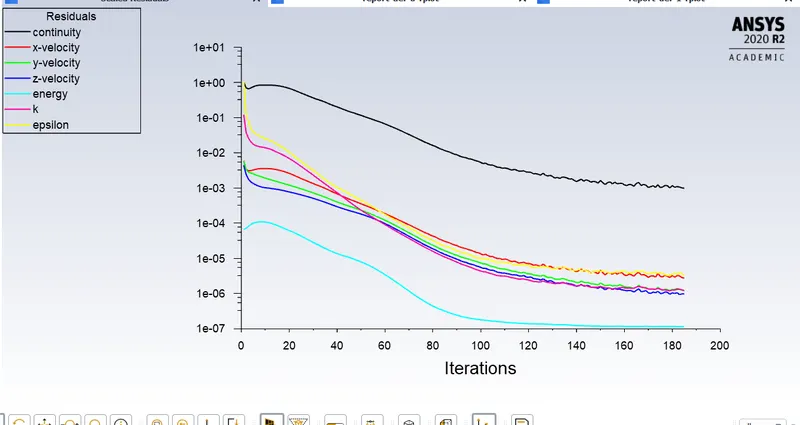
Residuals:

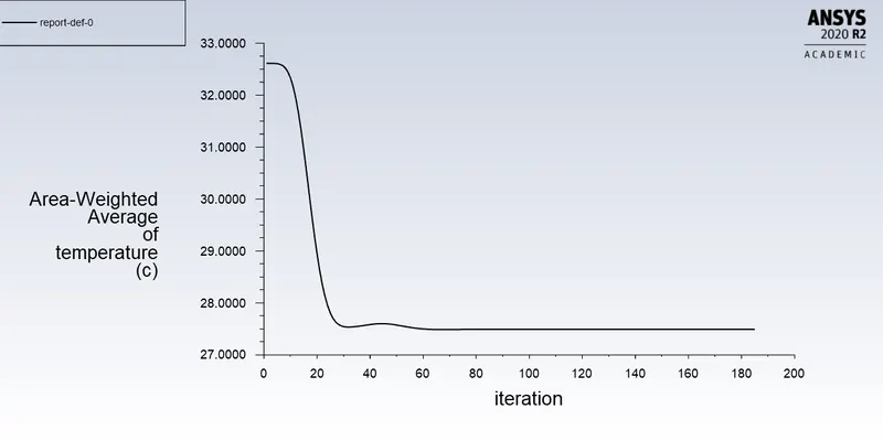
Average outlet temperature:

Standard deviation of temperature:

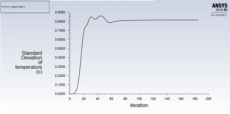
Temperature across the plane:

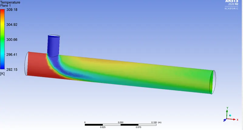
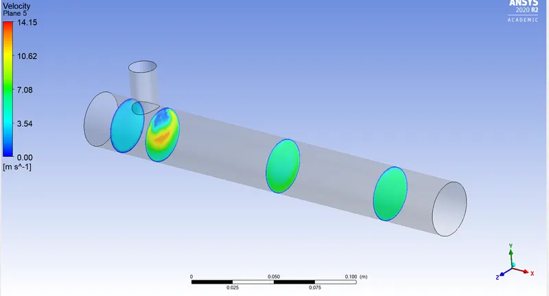
Velocity across the plane:

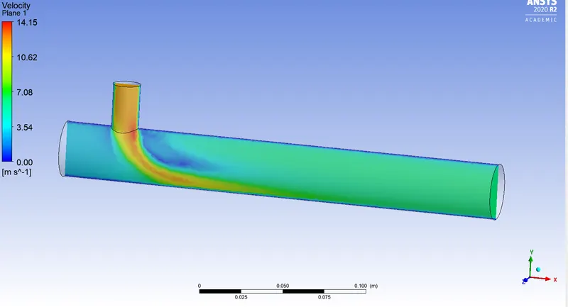
Velocity and temperature contour plots on the cut planes along and across the pipe:

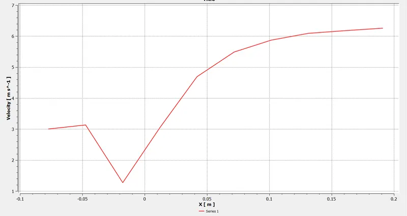
Velocity:

Temperature:

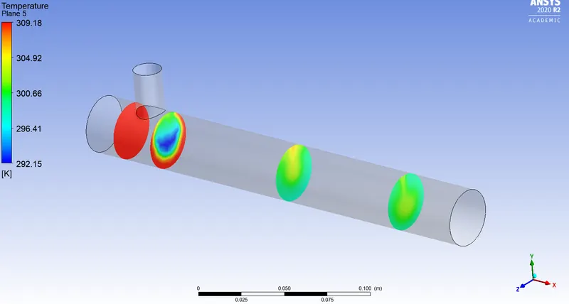
Temperature line plot:

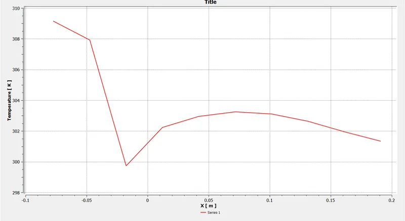
Velocity line plot:

*Long mixing tee with a hot inlet velocity of 3m/s and cold inlet velocity of 6 m/s using k-omega SST layer.

when hot inlet temperature is 36⁰C & the Cold inlet is at 19⁰C.

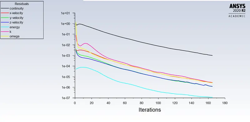
Residuals:

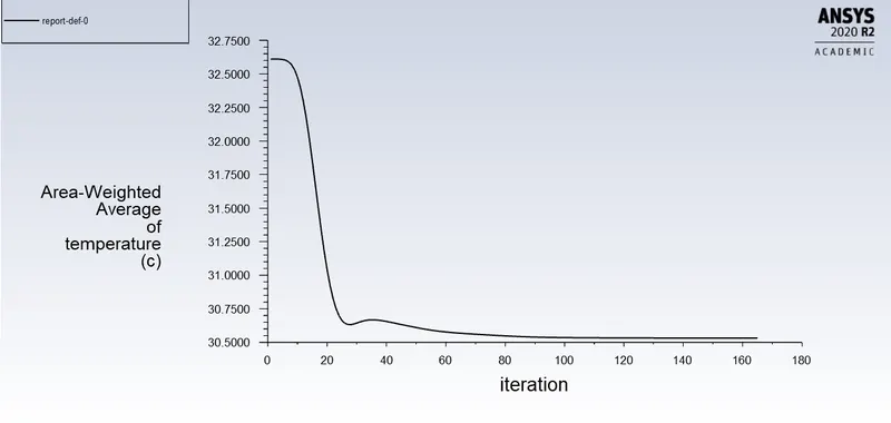
Average Outlet temperature:

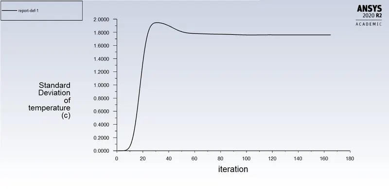
Standard deviation of temperature:

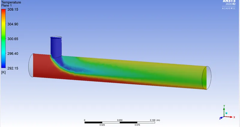
Temperature across the plane:

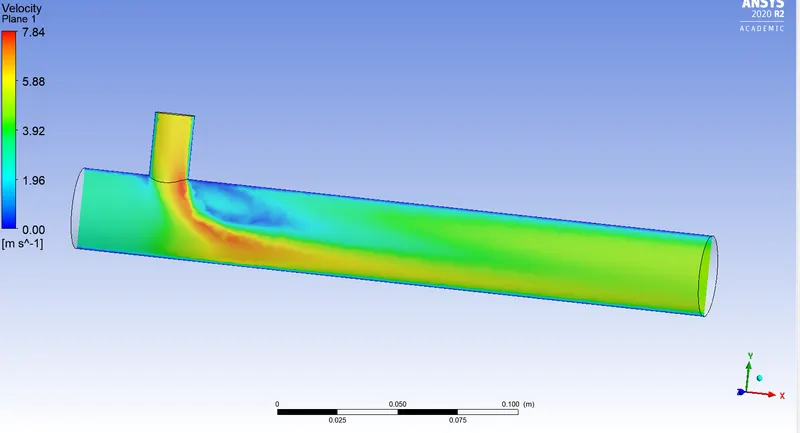
Velocity across the plane:

Velocity and temperature contour plots on the cut planes along and across the pipe:

Velocity:

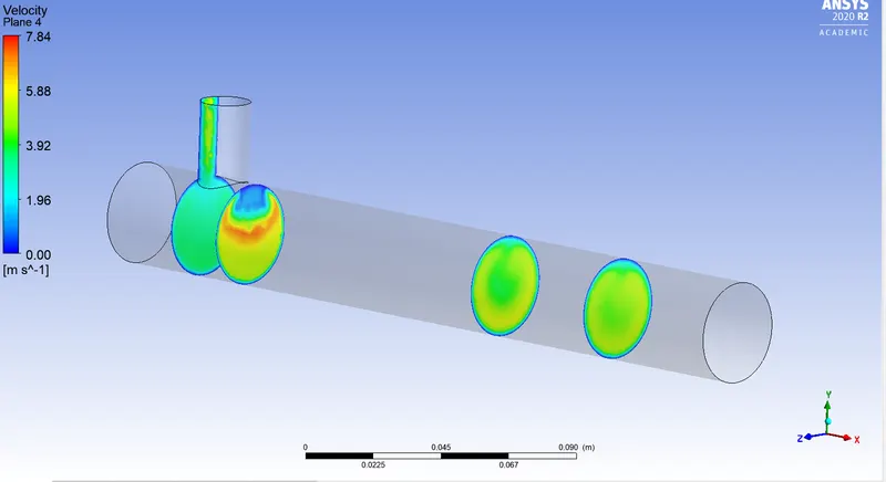
Temperature:

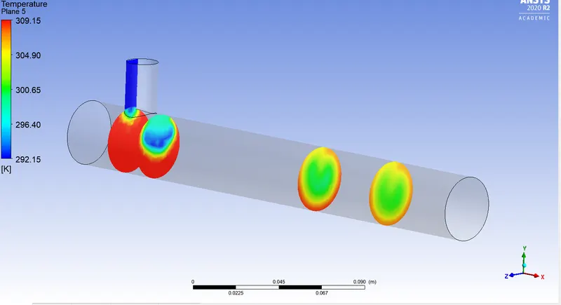
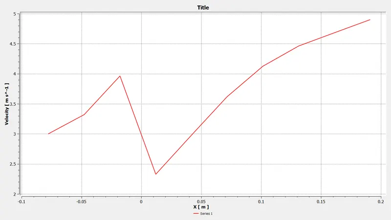
Velocity line plot:

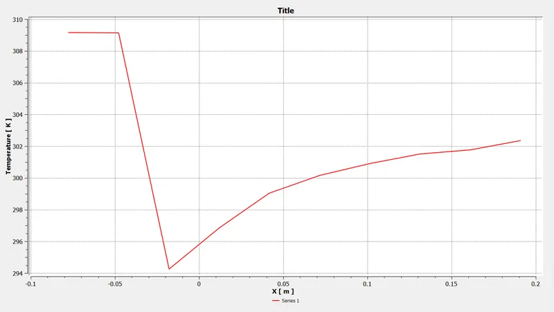
Temperature line plot:

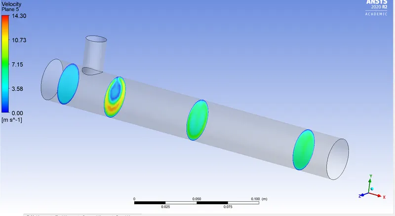
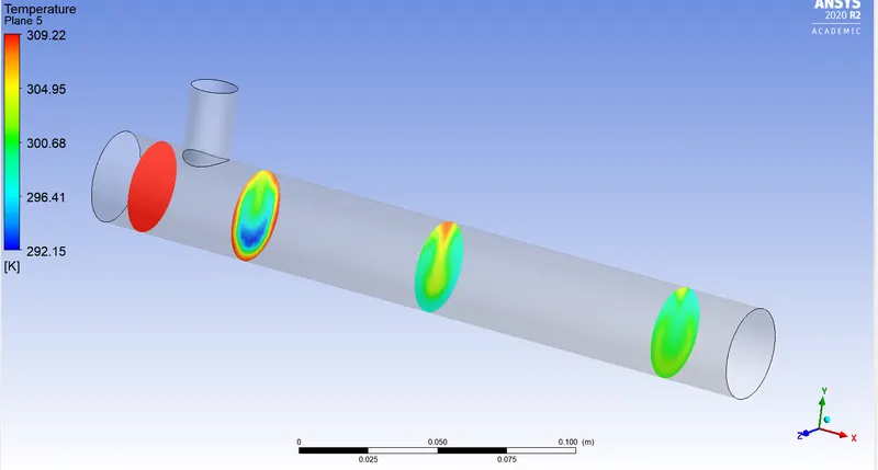
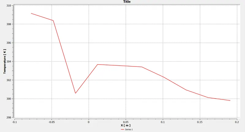
*Long mixing tee with a hot inlet velocity of 3m/s and cold inlet velocity of 12 m/s using k-omega SST layer.

when hot inlet temperature is 36⁰C & the Cold inlet is at 19⁰C.

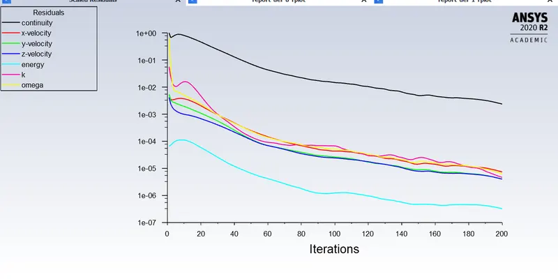
Residuals:

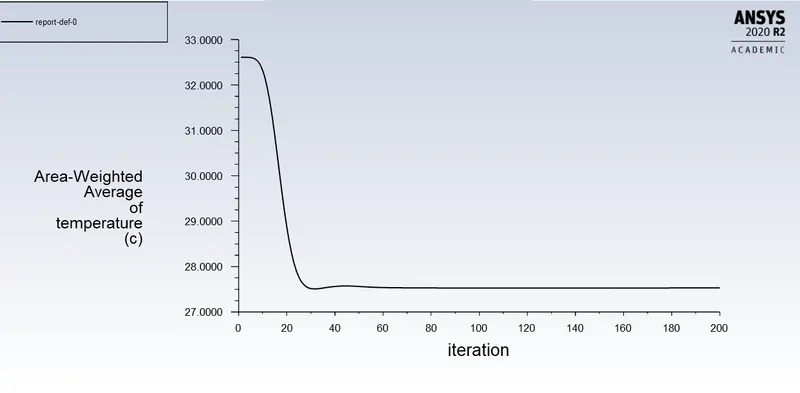
Average outlet temperature:

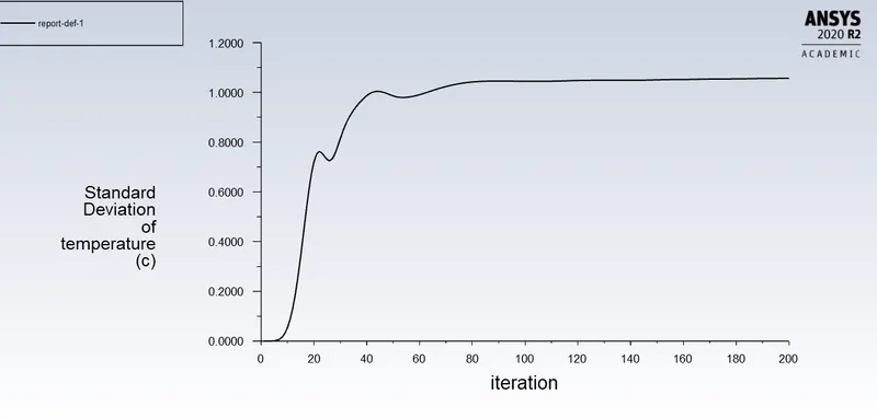
Standard deviation of temperature:

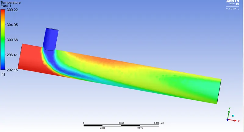
Temperature across the plane:

Velocity across the plane:

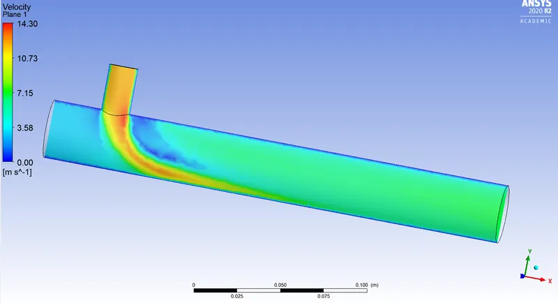
Velocity and temperature contour plots on the cut planes along and across the pipe:

Velocity:

Temperature:

Temperature line plot:

Velocity line plot:

Results:

case type Turbulence model standard deviation average outlet temperature iterations

short tee Realizable K-epsilon 1.75 30.30 160

(momentum ratio 2)

Short tee

(momentum ratio 4) Realizable K-epsilon 1.10 27.50 180

short tee K-omega SST 2.50 30.30 160

(momentum ratio 2)

Short tee

(momentum ratio 4) K-omega SST 1.50 27.50 190

long tee Realizable K-epsilon 1.30 30.30 175

(momentum ratio 2)

long tee

(momentum ratio 4) Realizable K-epsilon 0.81 27.50 185

long tee K-omega SST 1.8 30.70 168

(momentum ratio 2)

long tee

(momentum ratio 4) K-omega SST 1.05 27.50 200

Mesh independent study :

For element size default value 1.0219e-002m.

nodes-2797

elements-12583

Element size:2e-003m

Nodes:21407

Elements:106253

Element size 3e-003m

nodes:8306

elements:39510

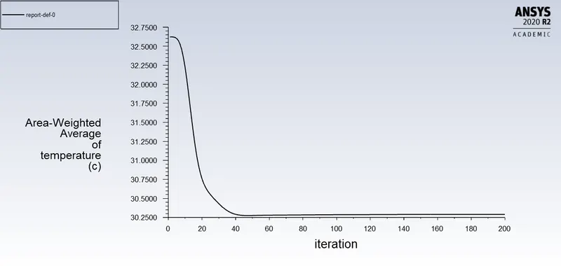
Here we can see clear convergence for element size 2.00e-003m.

Element size average outlet temperature

1.0219e-002m 30.30

3.00e-003m 30.30

2.00e-003m 30.25

Conclusion:

The resultant average temperature for both turbulence model Reliazable K -Epsilon & K omega SST looks similar, but for computing K omega SST takes more time and more number of iterations for convergence. Moreover, K epsilon predicts far from the boundary and K omega capture well near the wall also for the simulation we are dealing with the wall. high standard deviation means the mixing is bad and low standard deviation means the mixing is good chosing k -epsilon turbulence we get lower deviation,So I choose K - Epsilon Turbulence model.

For both case momentum ratio of 4, the outlet temperature drops significantly this occurs because of very high cold velocity air. So this clearly shows higher the momentum ratio greater the efficiency of the tee.

We are getting an almost similar result for short tee & long tee for the momentum ratio of 4 from this we can get to know that the length of the pipe doesn't affect the efficiency of the pipe.

When it comes to standard deviation, the long tee gives very lower value compared to the short tee. Indeed, we can increase high inlet cold air velocity for the application so we can get pretty good mixing in nature for a short pipe instead of using the long pipe.

If we increase velocity will get better turbulent mixing.majority of the mixing is because of higher velocity and as we go along the length of the pipe there is additional mixing that occurs because of diffusion.

Overall, the short tee pipe gives a pretty good result, and also it saves material cost. Increasing the pipe length doesn't create any difference in the outlet temperature.