Mixing efficiency

Objective :

To Simulate and understand steady-state mixing of two streamflow (one cold and hot) and hence calculate the effectiveness of the mixing. It is also studied how mixing length affects the effectiveness of mixing.

1. Case 1
   • Short mixing tee with a hot inlet velocity of 3m/s.
   • Momentum ratio of 2, 4.
2. Case 2
   • Long mixing tee with a hot inlet velocity of 3m/s.
   • Momentum ratio of 2, 4.

Here Momentum Ratio is defined as the Ratio of velocities of a cold and hot fluid stream.

`Momentum Ratio =( (Velocity)cold)/( (Velocity)hot)`

Mixing Tree simulation has a lot of significance in industrial applications like the HVAC systems, Nuclear Reactors, Chemical Reactors, Automobile industries, and many more. In this challenge, simulation has been done to understand the mixing efficiency of T- Joint flows.

Case 1 Setup:

Geometry: Short mixing tee

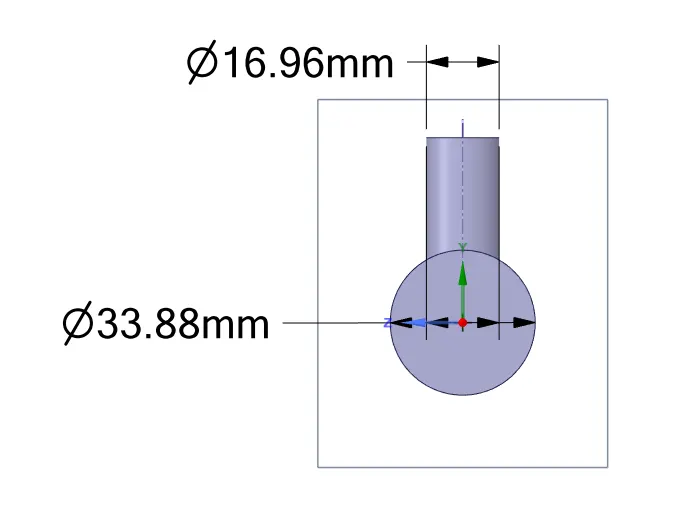
Fig 1: Side View of short mixing tree

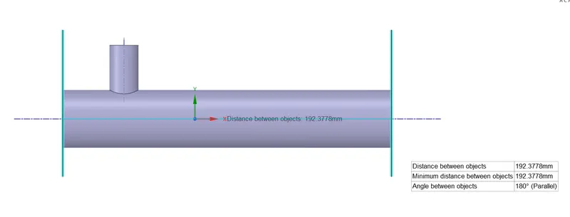
Fig 2: Front View of short mixing tree

The above geometry represents two streams of fluid, the left end of the pipe show an inlet pipe while the right end represents an outlet. There are two inlet pipes the shorter one for the cold stream while the other for the hot stream.

Mesh

Three Different sizes of mesh have been prepared to produce mesh independent solution.

1. Grid Size -- Default (10 mm)
2. Grid Size -- Default (3 mm)
3. Grid Size -- Default (1.2 mm)

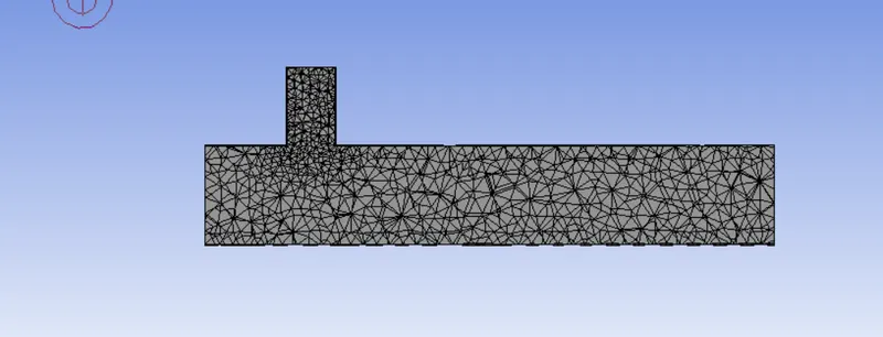
Fig 3: Sectional view of mesh generation

The quality of the mesh has been checked and listed below.

Fig 4: Mesh Quality

Named Selection: Inlet and outlet has been named for processing.

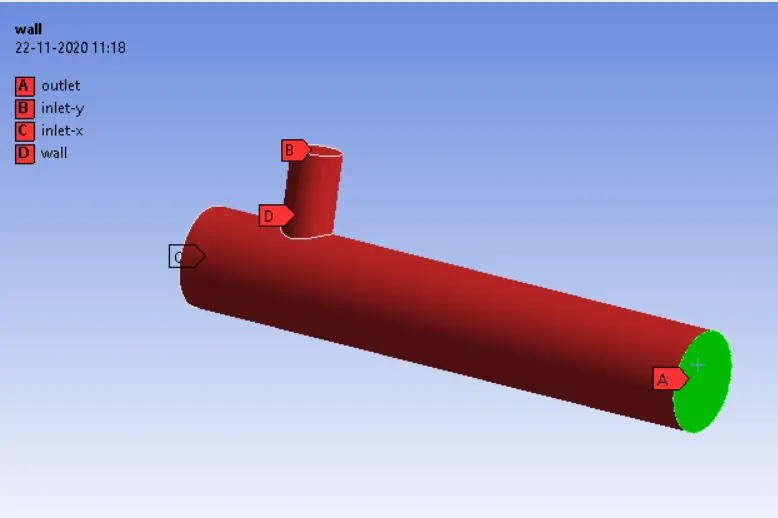
Fig 5: Name Selection

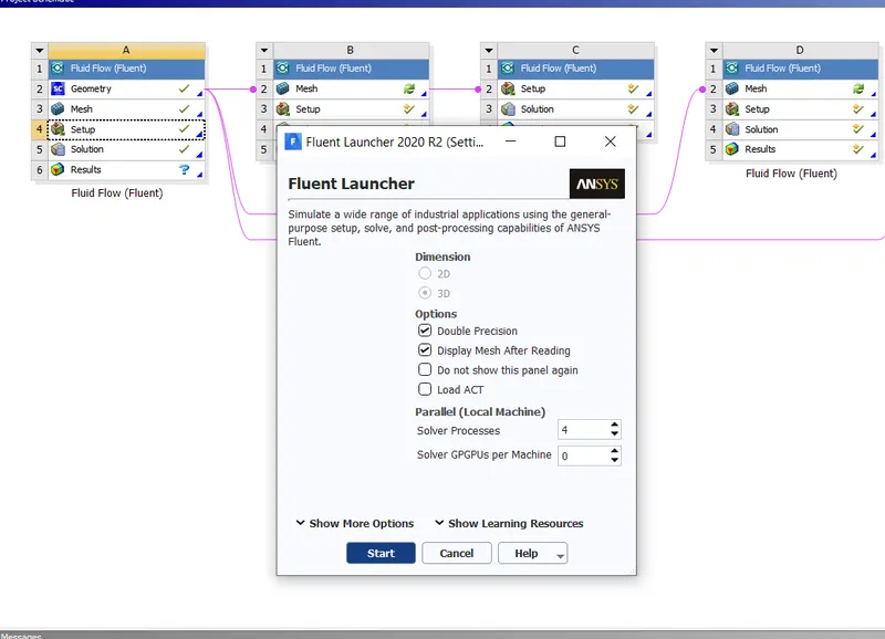
Fig 6: Setting dialogue box

Double Precision and 4 parallel processing have been selected for fast calculation.

Pressure Based steady-state solver has been selected for simulation. Since the density of the fluid is almost constant so Pressure based solver has been selected.

Since Temperature has to be solved so Energy has been turned on and since flow is in a turbulent region Therefore viscous, the k-epsilon model has been selected for simulation.

Inlet and Boundary Condition

Inlet_x Hot fluid Inlet

Velocity = 3 m/s, T= 36 `C`

Inlet_Y Cold Fluid Inlet

• Momentum Ratio = 2, V = 6 m/s T = 19 `C`
• Momentum Ratio = 4, V = 12 m/s T = 19 `C`

Outlet

Pressure based Gauge Pressure = 0 Pa

Wall

No slip Boundary condition imposed

Report Defination

• Area average Outlet Temperature
• Standard Deviation Outlet Temperature

Residue has been kept 1 e-06 for continuity, velocity, energy, k, and epsilon.

Result Plot:

Case 1: Short tree and 10 mm node size momentum Ratio =2

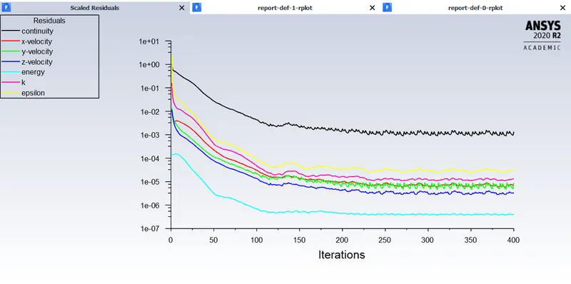
Fig7: Residue plot

Energy residue has reached 1 e-06 while others have not reached the limit.

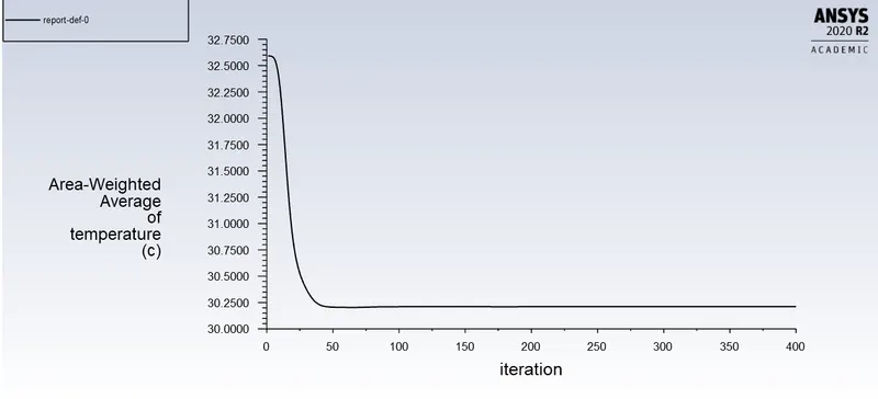
Fig 8: Area weighted average Temperature at Outlet

From the above plot, it is clear that after 80 simulation convergence has achieved because there is no fluctuation of temperature beyond that. The final Outlet Temperature is 30.25 C.

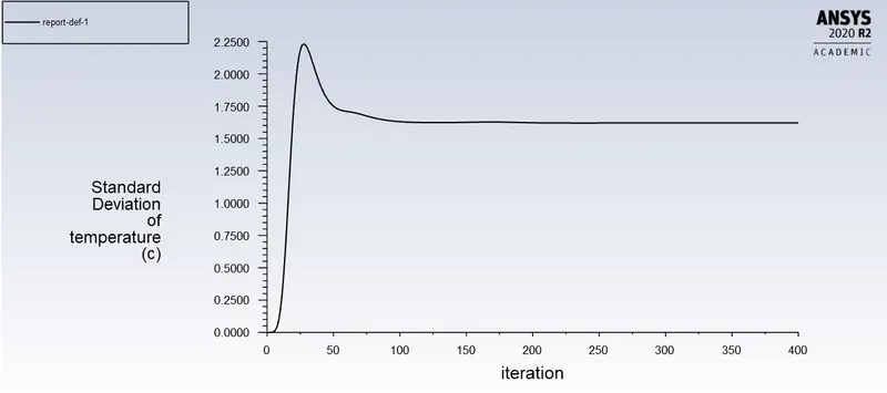
Fig 9: Standard Deviation of outlet Temperature

From the above plot, it is clear that after 80 simulation convergence has achieved because there is no fluctuation of Standard deviation of temperature beyond that. The final Standard deviation of temperature at the outlet is 1.7 C, This implies the mixing of the cold and hot fluid has 1.7C fluctuation at the outlet.

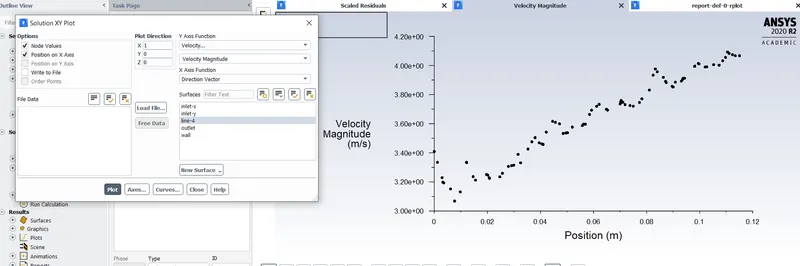
Fig 10: Variation of velocity at the central line

The Final velocity is approximately 4 m/s.

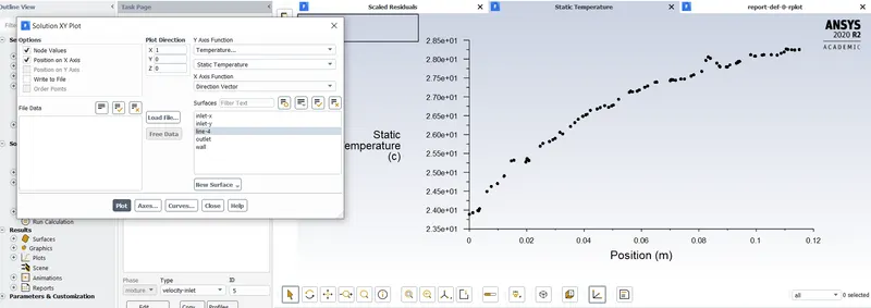
Fig 10: Variation of Temperature at the central line

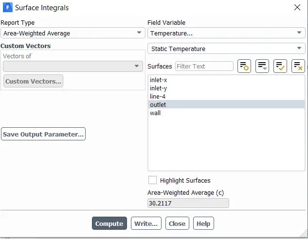
Fig 11: Area Weighted Average Temperature at outlet 30.217 C

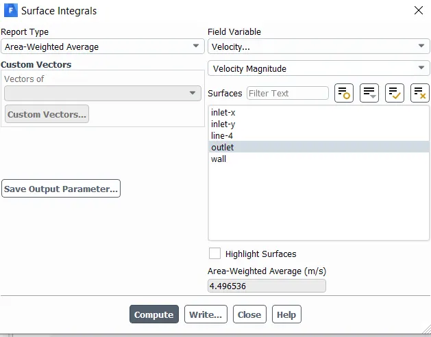
Fig 11: Area Weighted Average Velocity at outlet 4.49 m/s

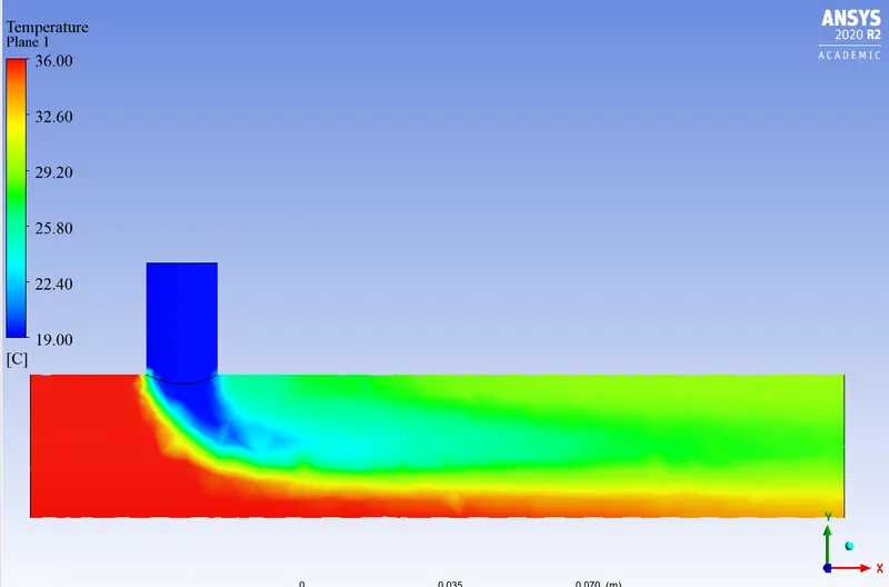
Fig 12: Temperature at the midplane

Since the mesh is coarse therefore there is a diffused temperature at the mixing junction.

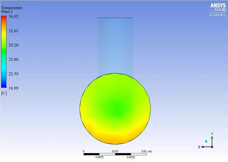
Fig 13: Temperature at the outlet stream

`Case 2: Short tree and 3 mm node size `

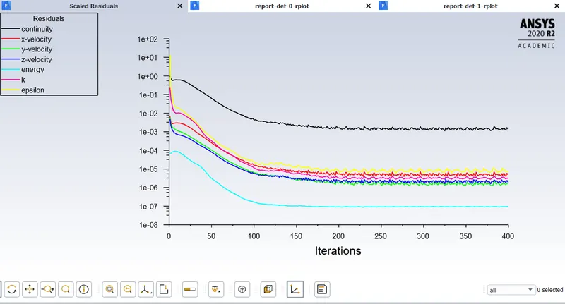
Fig14: Residue plot

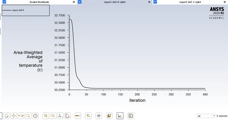
Fig 15: Area weighted average Temperature at Outlet

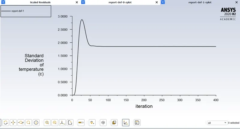
Fig 16: Area weighted Standard Temperature at Outlet

`Case .3: Short tree and 3 mm node size `

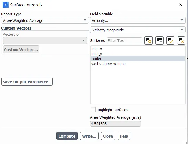
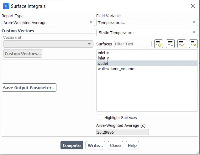
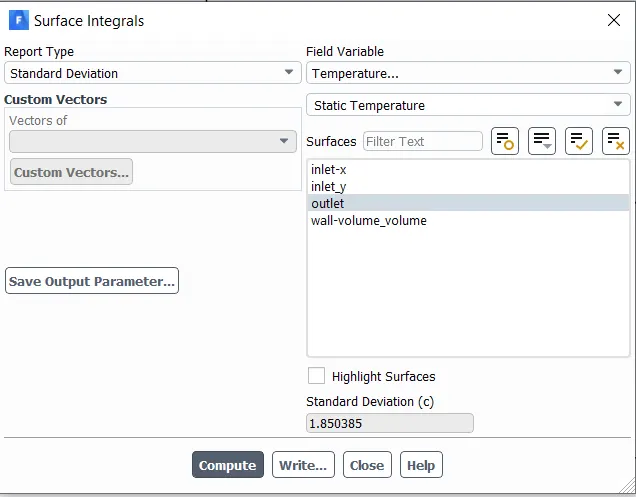
The area-weighted average of Velocity is 4.5 m/s while the area-weighted average of Temperature is 30.29 C and the Standard Deviation of Temperature is 1.8 C.

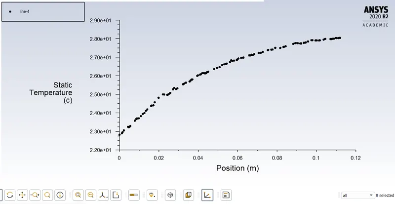
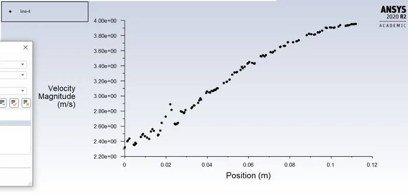
Temperature and Velocity variation along the central line

From the above two cases, it is clear the solution is mesh-independent. Differences in both cases are negligible.

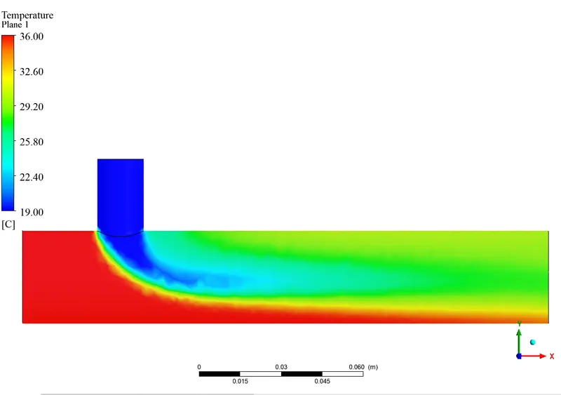
Variation in Temperature at mid-plane

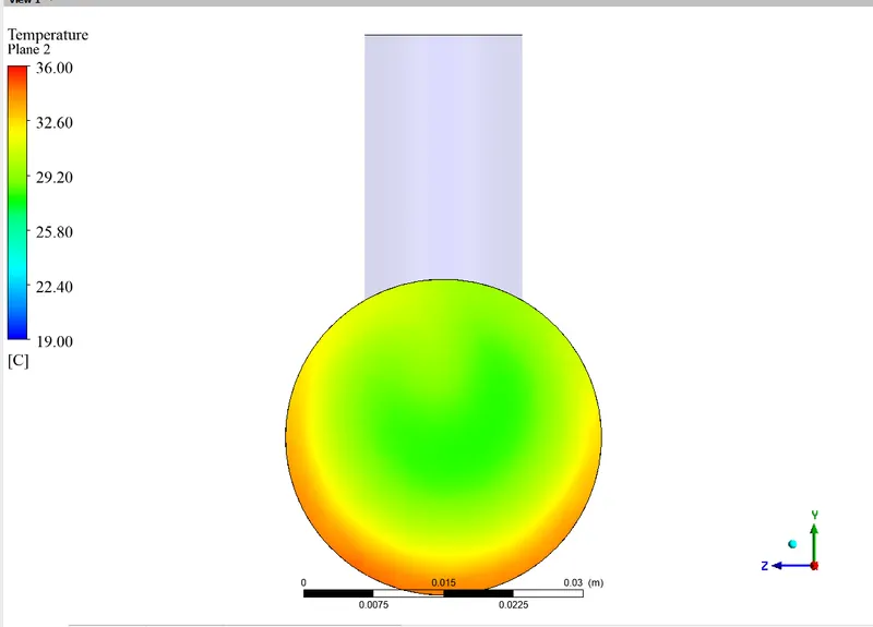
Variation in Temperature at outlet

Case 4: Short tree and 3 mm node size momentum Ratio =4

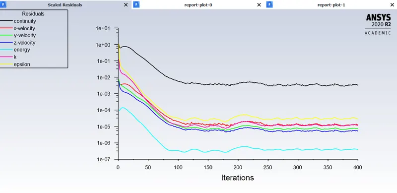
Residual plot

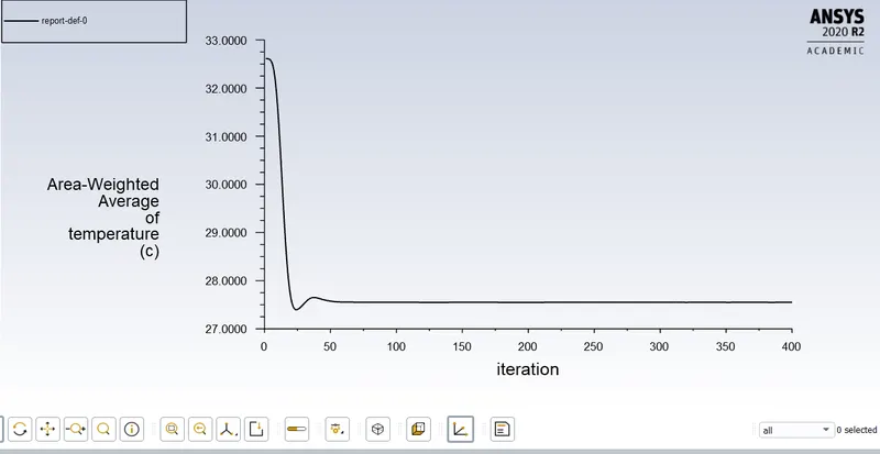
Area weighted average Temperature at the outlet

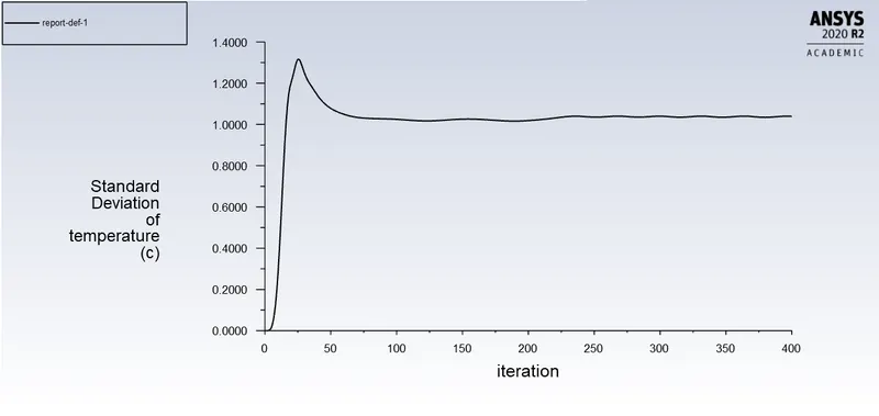
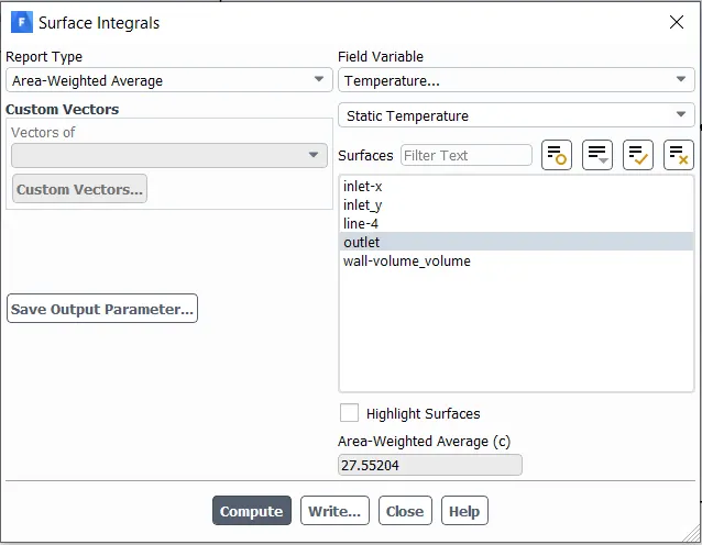
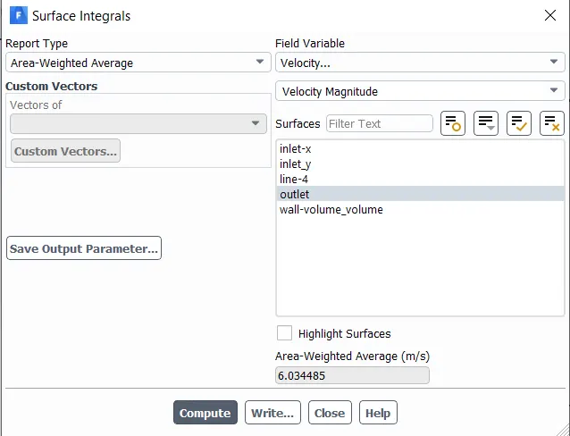
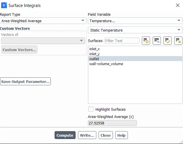
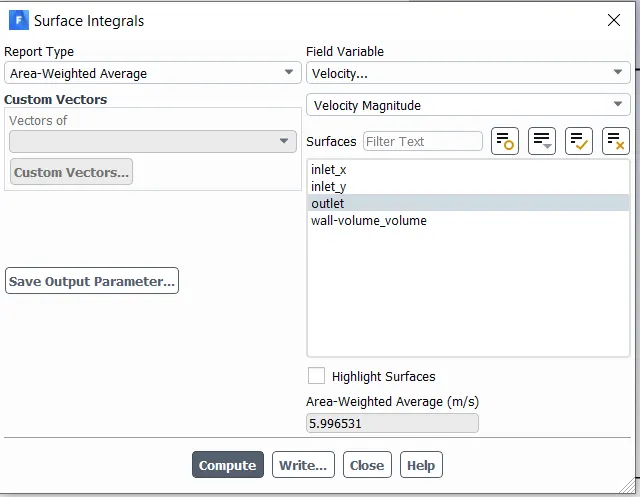
Average Temperature = 27.55 C Average Velocity at Outlet = 6.03 m/s

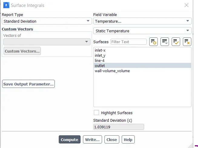
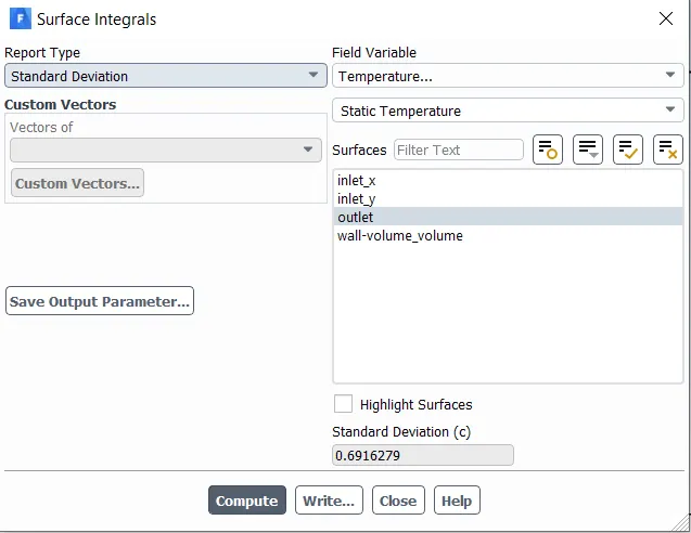
As the momentum ratio increases, there is better mixing at the outlet.

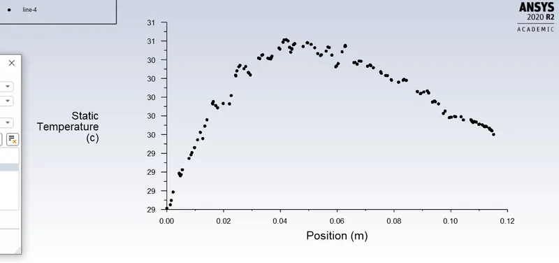
Variation of Temperature along the central line of the tube.

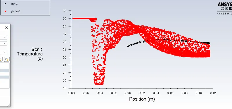
Comparative study of the mixing of the temperature at the central plane and central line

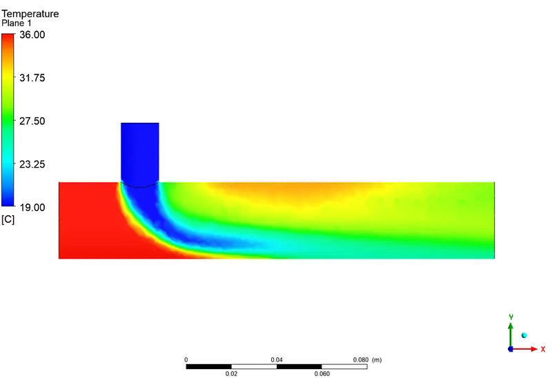
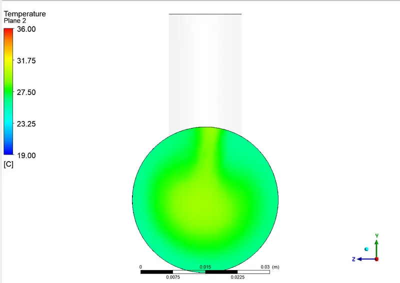
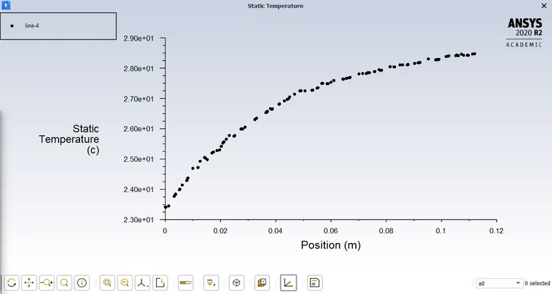
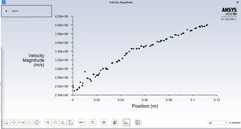
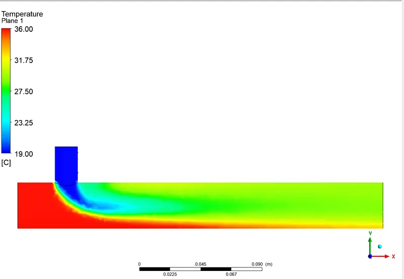
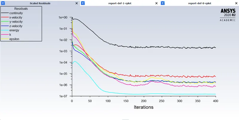
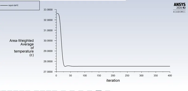
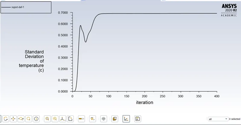
Case 5: long tree and 3 mm node size momentum Ratio =2

Conclusion:

Theoretical Calculation:

V_out = (m1*V1+m2*V2)/(m1+m2)

where m1 = `\rho1`*A1*V1

V_out = 4.01 m/s (For Momentum Ratio 2) V_simulation = 4.5 m/s

V_out = 6.03 m/s (For Momentum Ratio 4) V_simulation = 6.03 m/s

T_out = (m1*h1+m2*h2)/(m1+m2)*cp

Specific Enthalpy (@19 C)=292.552 KJ/kg
Specific Enthalpy (@36 C)=309.688 KJ/kg

T_out = 27.6 m/s (For Momentum Ratio 2) T_simulation = 30.29 m/s

T_out = 24.5 m/s (For Momentum Ratio 4) T_simulation = 27.55 m/s