CFD analysis of flow through Tee junction by using Ansys fluent

Abstract

This project involves the steady, incompressible analysis of the flow of air through Tee junction. Ansys fluent software is used to simulate the flow of air. The effect of length of the pipe after the junction and also the cold air inlet velocity is varied to investigate the effectiveness of the Tee junction. Turbulent models K-epsilon and K-omega SST model is used to simulate the flow through Tee junction. Both the k-epsilon and k-omega SST model gives good results and the results are validated by analytical results. An increase in the cold inlet velocity provides more mixing efficiency and an increase in pipe length help to reach thermal equilibrium.

Introduction

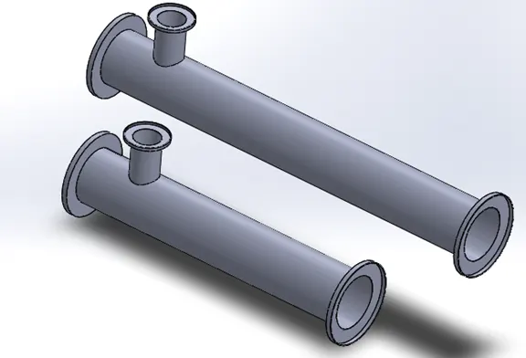
Tee Junction is the connection of two pipes of the same or different diameters generally used to mix two streams of fluid or dividing one stream of fluid into two. It has one straight pipe and another branch can be at any angle [1]. Tee junction is mainly used to mix two streams of water to get a required temperature at the outlet. This can be used in applications like HVAC, oil and gas industry, Nuclear reactors, etc. Two fluids mix and reach thermal equilibrium. The mixing efficiency depends upon the geometrical as well as flow properties. Efficient mixing results in the thermal equilibrium of the fluid at the outlet. Efficient mixing can be obtained if the length of the pipe is large enough to let the fluid mix together. But increasing the length of the pipe can increase the cost and material usage. Other methods for efficient mixing can be achieved by incorporating the components inside the pipe to divert the fluid direction, but it will increase the complexity of the design. In this project, computational fluid dynamics is used to evaluate the mixing efficiency of a Tee junction. Two Tee junctions of different length are taken for the analysis. Ansys fluent is used to analyze the flow through Tee junction. With the help of results found from the simulation, a suitable selection of the pipe length and velocity for better mixing of fluid can be decided.

Literature Review

Tee junction undergoes highly transient temperature fluctuations that can lead to security issues in the nuclear power plant. The thermal stresses generated in the pipe can cause thermal fatigue and finally failure of the pipe system. So it is important to predict the temperature distribution to take the appropriate precautions in Tee junctions [2]. A study conducted to find the suitable turbulent model for a flow of fluid through pipe showed that the k-epsilon turbulent model with enhanced wall function gives the accurate results to predict the friction factor among another turbulent model. K-omega SST turbulent model gives good accuracy in turbulent intensity in the pipe flow [3].

Problem Statement

Velocity and temperature details at the hot and cold inlet are shown in the table below. Mixing the effectiveness of the two Tee junctions of different length needs to be evaluated. The suitable turbulent model among k-omega SST and k-epsilon also needs to be identified.

Methodology

Since the thermal stress in the pipe material is not considered in this project only the fluid domain needs to be evaluated. Using Ansys Spaceclaime volume extraction, the fluid model can be selected. The cad model is meshed by tetrahedral mesh structure and to capture the boundary layer, inflation layers are used. The first layer thickness is calculated by keeping y+ = 1. The least layer thickness among the three sections needs to be selected. Three sections include the cold inlet, hot inlet, and the section after the mixing. Engineering Equation solver is used to solve the system. Hot inlet velocity is constant and cold inlet velocity is changing from 6m/s to 12m/s.

T[1] = 19[C] " Cold ait inlet temperatuire"

T[2] = 36[C] "Hot air inlet temperature"

P = 101.325[kPa] " Pressure"

rho[1]=Density(Air_ha,T=T[1],P=P) "Inlet cold air density"

h[1]=Enthalpy(Air_ha,T=T[1],P=P) "inlet cold air enthalpy"

rho[2]=Density(Air_ha,T=T[2],P=P) "Inlet hot air density"

h[2]=Enthalpy(Air_ha,T=T[2],P=P) "Inlet hot air enthalpy"

V[1] = 6 [m/s] "Inlet cold air velocity"

V[2] = 3 [m/s] "Inlet hot air velocity"

D[1] = 0.017 [m] "Inlet cold Diameter"

A[1] = 3.14/4*((D[1])^2) "Inlet cold side area"

D[2] = 0.0339[m] "Inlet hot side Diameter"

D[3] = D[2] "Outlet DIamerter"

A[2] = 3.14/4*((D[2])^2) "Inlet hot side area"

A[3] = A[2] "Outlet side area"

m[1] = A[1]*V[1]*rho[1] "Cold air mass flow rate"

m[2] = A[2]*V[2]*rho[2] "Hot air mass flow rate"

m[3] = m[1]+m[2] "Outlet mass flow rate"

h[3] = (m[1]*h[1]+m[2]*h[2])/m[3] "Outlet air enthalpy"

T[3] =Temperature(Air_ha,h=h[3],P=P) "Outlet air temperature"

rho[3]=Density(Air_ha,T=T[3],P=P) "Outlet air density"

V[3] = m[3]/(rho[3]*A[3]) "Outlet air velocity"

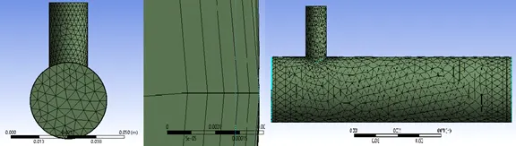
Considering the velocities 3,6, 12, and 13.33 the minimum cell thickness for y+ =1 will give the first boundary layer cell from the surface. The cell thickness decreases with velocity and the first cell thickness obtained (https://www.pointwise.com/yplus/) is 0.00002m. Thus the first inflation layer will have a height of 0.02mm. The final mesh structure is shown below.

A grid dependency test is performed for both short and long Tee junction pipes. The elements, nodes, and the converged velocity and temperature at the exit are shown below.

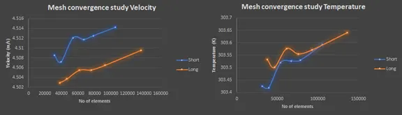
An increase in the number of mesh elements changes the outlet temperature and velocity. The change is found out to be less and is in the range of 0.05K for temperature and 0.002m/s for velocity. Thus the number of nodes and elements that can be used in the analysis for the short and long pipe is shown below.

	Nodes	Elements
Short	19234	54030
Long	26803	75965

Since the analysis is to find the effectiveness of the Tee junction, the final temperature at the exit needs to be evaluated. Steady-state analysis and the pressure-based solver has to be used. Boundary conditions are velocity at both inlets and outlet pressure is atmospheric. At walls, no-slip boundary conditions are applied. Solution methods involve simple pressure velocity coupling and second-order discretization is used in pressure gradient. Turbulent dissipation rate and turbulent kinetic energy terms are discretized by the first-order upwind method. Momentum and energy terms are iterated by using second-order terms. Hybrid initialization is used to find the initial conditions in the system.

Results & Discussion

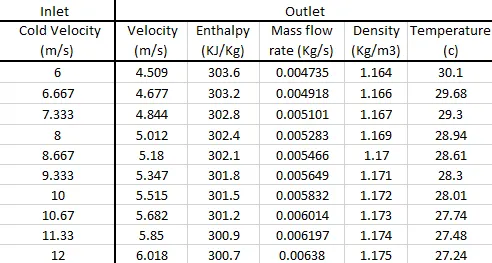
The table shows the air velocity and temperature at the exit of the Tee junction.

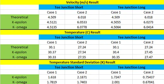
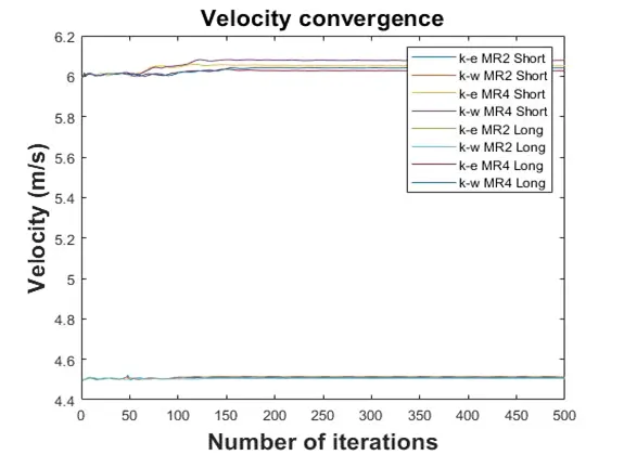
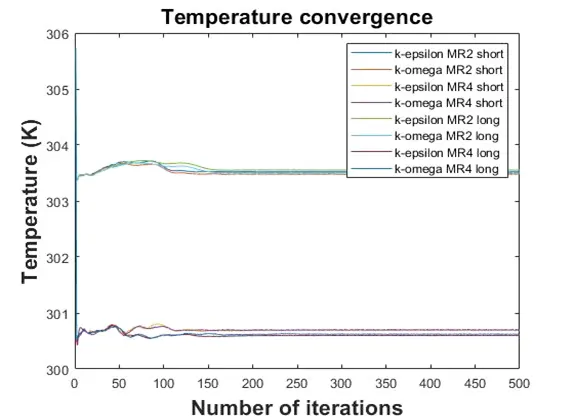
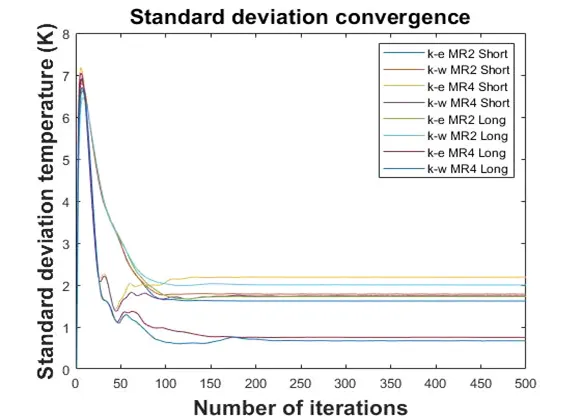
Velocity results show that the K-epsilon turbulent model predicts the flow velocity and the outlet velocity matches the theoretical result. The K-omega turbulent model also gives close results but the error in predicting the exit velocity is more in the result, obtained by using the k-omega turbulent model. The error increases with the flow velocity. In the case of temperature results, both turbulent models give a matching result, but the k-omega SST turbulent model gives a close result. The temperature standard deviation shows that the k-omega model predicts temperature accurately at high-velocity mixing conditions. All the simulations converged in less than 200 iterations. All the parameter values after 200 iterations changes in negligible rate.

Convergence Plot

Velocity Contour Plots along the flow direction

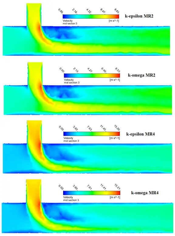
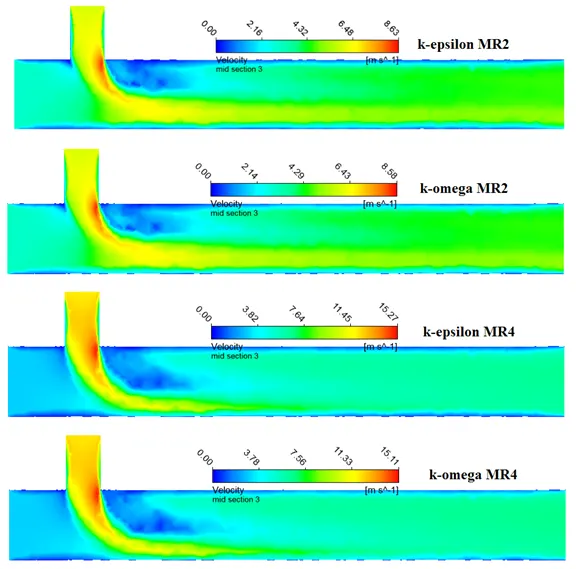
The velocity gradient at the wall surface is visible in the k-epsilon model. But far from the boundary, the velocity profile has no change in both turbulent models. The mixed flow at the exit is observed when the cold fluid inlet velocity is increased. Even though the result at the exit from both turbulent models is matching the k-epsilon turbulent model gives a clear profile inside the pipe. As the cold inlet velocity increases the mixing is more efficient.

Shorter pipe

longer pipe

Temperature Contour Plots along the flow direction

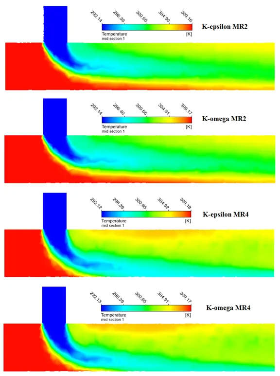
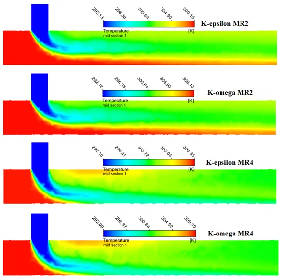
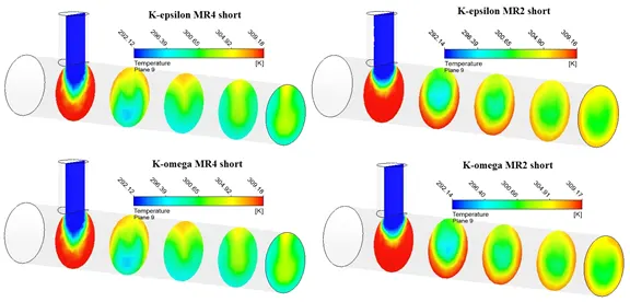
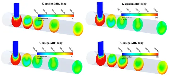
K-omega SST turbulent model gives close matching temperature results with the theoretical values. Mixing efficiency is increases with the increase in the cold inlet velocity; The difference between the theoretical value of temperature and the simulation result decreases with the increase in the cold inlet velocity. Due to the increased mass flow rate, the temperature at the exit is reduced in case 2. Temperature diffusion is increased in case 2 where the cold inlet velocity is more.

Shorter pipe

Longer pipe

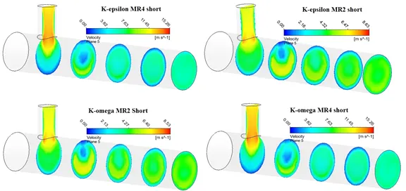
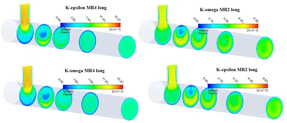
Velocity Contour Plots across the flow direction

The plots shown below shows the cross-section profile at a different location along with the flow. The cross-sectional profile obtained from both turbulent models is matching each other except at the wall boundary.

Temperature Contour Plots across the flow direction

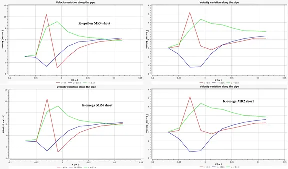
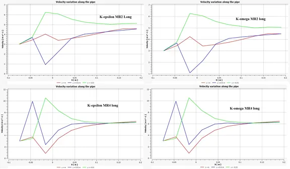
Velocity line Plots along the flow direction

The temperature along the pipe at three locations are observed. In the cases when the cold air inlet velocity increases the velocity at exit locations reaches the same velocity magnitude. It means that the increase in the inlet cold velocity provides efficient mixing.

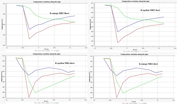
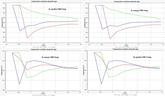
Temperature line Plots along the flow direction

The temperature at the locations is not the same even if the velocity is increased. It is seen that for longer pipe the thermal equilibrium reached provided the inlet cold velocity is increased. For longer pipe the flow getting the time to reach thermal equilibrium.

Conclusion

1. Increase in the momentum ratio thereby cold inlet velocity temperature increases the mixing efficiency.

2. Increase in the length allows the two streams of flow to reach thermal equilibrium provided the cold inlet temperature is increased.

3. Both k-epsilon and k-omega SST model is good at predicting the velocity and temperature and the results are matching with the theoretical results with a maximum of 1.3% error.

4. Even though the changes are very less, the k-epsilon turbulent model gives accurate results compared to the k-omega SST model in the analysis.

Velocity Error (%) Result
	Tee Junction Short		Tee Junction Long
K-epsilon	0.068751386	0.586573612	0.077622533	0.154536391
K- omega	0.099800399	0.99368561	0.057662453	0.3888335
Temperature Error (%) Result
K-epsilon	0.897009967	1.101321586	0.996677741	0.77092511
K- omega	0.764119601	1.138032305	0.830564784	0.844346549

References

[1] J. Štigler, R. Klas and O. Šperka, "Characteristics of the T-junction with the equal diameters of all branches for the variable angle of the adjacent branch", EPJ Web of Conferences, no. 67, pp. 1 - 12, 2014. Available: 10.1051/epjconf/20146702110 [Accessed 10 October 2020].

[2] T. Frank, C. Lifante, H. Prasser, and F. Menter, "Simulation of turbulent and thermal mixing in T-junctions using URANS and scale-resolving turbulence models in ANSYS CFX", Nuclear Engineering and Design, vol. 240, pp. 2313 – 2328, 2009. Available: 10.1016/j.nucengdes.2009.11.008 [Accessed 10 October 2020].

[3] D. C. Lim, H. Al-Kayiem, and J. C. Kurnia, "Comparison of Different Turbulence Models in Pipe Flow of Various Reynolds Numbers", AIP Conference Proceedings, no. 2035, pp. 1 - 9, 2018. Available: 10.1063/1.5075553 [Accessed 10 October 2020].