Matlab PROJECT to describe the solution of SECOND ORDER ORDINARY DIFFERENTIAL EQUATIONS.

AIM : To write a program in Matlab to Visualize and Understand the Concept of Solving Second Order ODE of a Simple Pendulum.

INTRODUCTION :

BRIEF INTRODUCTION ON DIFFERENTIAL EQUATIONS :

Differential Equation is an equation that contains the function and its derivatives.In a more simpler way we can justify the equation to be differential equation, if it contains any derivative.

Differential Equations are basically classified based on the order and degree.

ORDER is the number of the highest derivative in a differential equation.

DEGREE : The degree of differential equation is represented by the power of the highest order derivative in the given differential equation.It is described in the folowing table:

Highest Derivative in the DE	Order of DE	Degree of DE	Description
`dy/dx`	1	1	First Order First Degree Differential Equation
`((d^2y)/dx^2)^2`	2	2	Second Order Second Degree Differential Equation
`(d^3y)/dx^3`	3	1	Third Order First Degree Differential Equation

Solution Of Differential Equation :It is nothing but the the function `y=f(x)`

In order to find the function `y=f(x)`,various methods are adopted depending on the type of Differential Equation.For high calculations and for high range of values we cannot implement manual calculations.So the softwares do that work.Many softwares solve the Ordinary Differential equations using various ode solvers.One of such a solver used by the Matlab software is ode45.In this project we will be discussing about ode45 and it's application to solve the Ordinary Differential equations by considering an example of simple pendulum.

BRIEF INTRODUCTION OF ODE45 SOLVER :

ODE45 is a Matlab Command that performs a direct numerical integration of a set of differential equations `y'=dy/dx=f(x,y)`, from initial time(`t_i`) to final time(`t_f`).

ODE45 is so called because this command implements the Numerical method called Runge-Kutta(4,5) Method to solve the Differential method.

SYNTAX OF ODE45 :

[t,y] = ode45(odefun,tspan,y0)

Here,

• `tspan = [[t_0, t_f]]` is a row matrix containing all the values of 't' for which the value of 'y' need to be found out .
• `[t,y]`= Here 't' is the column vector containing the values of 't' for which the values of 'y' are calculated.Here 'y' is the solution array in which each row corresponds to the values of each row in column vector 't'.
• odefun= It indicates the differential equation that are solved.Various Parameters that are included in the function are sent from the main function for evaluation.
• `y_0`= It is the column matrix of Initial Values.

BRIEF INTRODUCTION OF RUNGE-KUTTA METHOD OF 4TH ORDER :

It is an numerical approach to solve a Differential equation and find out the approximate values of the function.This method uses an iterative method to find the solution until a desired level of accuracy is achieved.

The following formulas describe the method:

`y'=F(x,y)` where `y=f(x)impliesy_0=f(x_0)`

`y_(n+1)=y_n+1/6(k_1+2k_2+2k_3+k_4)`

where,

`k_1=hF(x_n,y_n)`

`k_2=hF(x_n+h/2,y_n+k_1/2)`

`k_3=hF(x_n+h/2,y_n+k_2/2)`

`k_4=hF(x_n+h,y_n+k_3)`

Here h=stepsize which changes during each iteration.Every time a new value of 'y' is calculated for a new value of 'x' .

The ode solver takes the Function F(x,y) and the initial conditions to calculate the solution array for different values of x.

In this project we consider a case of a simple pendulum to depict its angular displacement and angular velocity from the differential equation that is solved by ode45.This is done using Matlab Programming Language.The animation is also created in the Matlab to Visualize the Oscillatory motion of a simple pendulum.

BRIEF INTRODUCTION OF SIMPLE PENDULUM :

A point mass attached to a light inextensible string and suspended from fixed support is called a simple pendulum.It consists of a bob of mass 'm' suspended through a string of length 'L' pivoted at a fixed point 'P', and subjected to oscillation.The following figure depicts the simple pendulum:

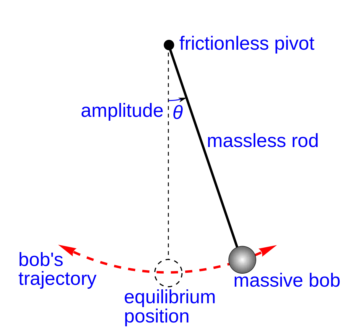
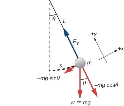
The bob of the pendulum is displaced by an angle `theta`and is subjected to continuous oscillations.The bob starts oscillating continuously and due to air friction and gravity the bob slowly starts to reach equillibrium position.

There are two basic forces acting on the bob of pendulum.They are:

• Tension Force of the string,always acting towards the pivot.
• Weight of the Bob acting vertically downwards.

When the bob is at extreme position,The Weight 'mg' of the bob gets resolved into two components :

1) `-mgsintheta`

2)`-mgcostheta`

The second component `-mgcostheta` is balanced by the Tension Force(`F_T`).The unbalanced component `-mgsintheta` tends to bring the bob back to equilibrium position and hence the bob starts to come back to the equilibrium position.Similarly at the other end also the force component `mgsintheta` tends to bring the bob back to equilibrium position.Thus the pendulum gradually reaches the equillibrium position and goes to rest.

When the bob reaches the equillibrium position the Velocity is said to be maximum and at the extremeties the velocity reduces to zero.

Similarly displacement is maximum at the extreme positions and minimum at the equillibrium.The differential equation describing the damping motion of a pendulum is given below:

`(d^2theta)/dt^2 + b/m(d theta) /dt +g/Lsintheta =0`

Here , g=Acceleration due to gravity(`m/s^2`)

m=mass of the bob(kg)

b=Damping Co-Efficient=It is the Damping Force per unit velocity (`(Ns)/m`).

L=Length of the string of a pendulum (m).

`theta`=Angular Displacement (rad)

`(d theta)/dt` = Angular Velocity (rad/sec).

OBJECTIVES :

• To Understand the concept of working and syntax of ODE45 solver using Matlab .
• To plot a graph to show the variation of Angular Displacement and Angular Velocity of a simple pendulum with respect to time using ode solver.
• To create an animation describing the oscillatory motion of Simple Pendulum using Matlab.

GOVERNING EQUATIONS :

`(d^2theta)/dt^2 + b/m(d theta) /dt +g/Lsintheta =0` having `theta=0` and`(d theta)/dt=3`m/s at time,t=0 `

Here , g=Acceleration due to gravity(`m/s^2`)

m=mass of the bob(kg)

b=Damping Co-Efficient=It is the Damping Force per unit velocity (`(Ns)/m`).

L=Length of the string of a pendulum (m).

`theta`=Angular Displacement (rad)=Shortest Angle between the vertical and the string Length.

`(d theta)/dt` = Angular Velocity (rad/sec).

This is a Second order Differential Equation.In order to solve this we need to convert this second order differential equation into First order Differential Equations.This is done as follows:

The differential equations are given as:

`d/dt((d theta)/dt)+ b/m(d theta) /dt +g/Lsintheta =0`

The two First order Differential Equations are:

1. `(d theta)/dt =theta_1`
2. `(d theta_1)/dt=-b/m(theta_1)-g/lsintheta`

These two equations are written in the ode_func and thus the solution array is calculated.

Equations to plot the co-ordinates:

`x=Lcos(pi/2-theta)` `implies x=Lsintheta`

`y=-Lsin(pi/2-theta)` `implies y=-Lcostheta`

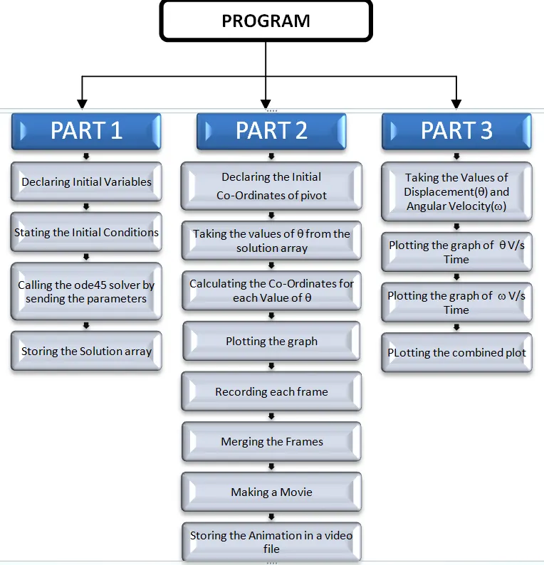
FLOW CHART DESCRIBING THE FLOW OF COMMANDS :

MATLAB PROGRAM TO PLOT AND ANIMATE THE SIMPLE PENDULUM :

clear all
close all
clc
b=0.05;
m=0.1;
l=1;
g=9.81;
% PART 1 OF THE PROGRAM
% Initial conditions Where Displacement=0 and Velocity=3 m/s 
theta_1=[0;3];
% Total time
t_span=linspace(0,20,500);
% Calling the ode45 solver and getting the solution array
[t,results]=ode45(@(t,theta)ode_func(t,theta,b,g,l,m),t_span,theta_1);
% PART 2 OF THE PROGRAM
% Co-ordinates of thePivot
x0=0;
y0=0;
% Counter variable
ct=1;
for i=1:length(t) 
    x1=l*sin(results(i,1));
    y1=-l*cos(results(i,1));
    plot([-l l],[0 0],[x0 x1],[y0 y1],'-o','color','r','linewidth',3,'markerfacecolor','b','markersize',20);
    axis([-2,2,-2,2]);
%     Recording and storing the frames in array M
    M(ct)=getframe(gcf);
    ct=ct+1;
end
% Merging the frames and Making a Movie
movie(M);
% Creating a Video file in .avi format
videofile=VideoWriter('Simple_Pendulum_Animation.avi');
% Opening a videofile
open(videofile);
% Writing the animation to the videofile
writeVideo(videofile,M);
% Closing the videofile
close(videofile);
% PART 3 OF THE PROGRAM
figure(1)
% Graph of Angular Displacement V/s Time
plot(t,results(:,1),'linewidth',2);
xlabel('time(sec)');
ylabel('displacement(rad)');
pause(1);
figure(2);
% Graph of Angular Velocity v/s time
plot(t,results(:,2),'color','r','linewidth',2);
xlabel('time(sec)');
ylabel('Angular Velocity(rad/sec)');
pause(1);
% Combined Plot
figure(3);
plot(t,results,'linewidth',2);

FUNCTION TO SOLVE DIFFERENTIAL EQUATION :

% Function Definition of odefunc
function [dtheta_dt]=ode_func(t,theta,b,g,l,m)
     theta1=theta(1);
     theta2=theta(2);
%      Finding the two second order ODE's
     dtheta1_dt=theta2;
     dtheta2_dt=-(b/m)*theta2 -(g/l)*sin(theta1);
%      Storing the results into a solution array
     dtheta_dt=[dtheta1_dt;dtheta2_dt];
end

DETAILED EXPLAINATION OF THE CODE :

The program is basically divided into three parts for better understanding:

1. PART 1 :Solving the Differential equation.
2. PART 2 :Making the Animation of Simple Pendulum.
3. PART 3 :Plotting the Graphs.

The code is explained in detail in the following steps:

PART 1 :

1. The program starts with clear all,close all and clc to clear the previous data from the command window.
2. Initially the variables such as Length of the string(l),acceleration due to gravity(g),Damping Co-Efficient(b),mass of the bob(m) are defined.
3. The initial conditions such as the angular displacement and the angular velocity at time t=0 sec, of the differential equation are defined in a column vector called 'theta_1'.This is given in the statement,theta_1=[0;3].
4. The total time span for integration is given by:'tspan=linspace(0,20,500).
5. Here the t_span is an array of 500 values between t=0 and t=20.The equal spacing is done using linspace command.
6. Now all the variables are ready to be sent as parameters to ode45 solver.
7. [t,results]=ode45(@(t,theta)ode_func(t,theta,b,g,l,m),t_span,theta_1): This is the command to solve the differential equation.
8. @(t,theta) indicates that Differential Equation is in terms of t and theta.
9. ode_func(t,theta,b,g,l,m) indicates the function containing the first order ODE to be solved.The parameters sent to the function are t,theta,b,g,l,m.
10. The brief Explanination of the function ode_func(t,theta,b,g,l,m) is given as follows:
11. This function is defined as ode_func and is saved in the same folder where the main program is saved.
12. In order to solve the Second order Differential Equations we need to convert them into two first order differential equations and then simplify.This is done in the function ode_func.
13. This function is executed for all 500 values of t_span.
14. The Solution array is stored in column vector dtheta_dt.This Column Vector is assigned to the results variable.
15. results is a matrix that contains 500 rows and 2 columns,Where the first column gives the values of Angular Displacement and the Second Column gives the values of angular Velocity.
16. In the above 7th step, variable t includes the time array for which the results matrix is calculatetd.
17. Each value of t corresponds to the each value in results array .

PART 2 :

1. Initial the Co-ordinates of the pivot are fixed at the origin.Therefore `x_0=0` and `y_0=0`.
2. Counter variable(ct) is assigned as 1.
3. The for loop is written for iteration for all 500 values of i and the 500 co-ordinates are calculated.
4. In order to get the x-co-ordinate the code is: x1=l*sin(results(i,1));
5. This is nothing but the projection of length l on to x-axis at an angle results(i,1).
6. Since we need each value of displacement in each iteration ,the code is written as results(i,1).The following table indicates the value of i and Displacement for six iterations.

7. Value of i	1	2	3	4	5	6
   Value of results(i,1)	results(1,1)	results(2,1)	results(3,1)	results(4,1)	results(5,1)	results(6,1)
   Angular Displacement	0	0.1187	0.2333	0.3419	0.4432	0.5358

8. The first seven rows of result matrix are shown below:
   results=[ 0 3.0000
   0.1187 2.9172
   0.2333 2.7910
   0.3419 2.6250
   0.4432 2.4237
   0.5358 2.1923
   0.6186 1.9360]
9. result(1,1) gives the value present in first row,first column of the results matrix i.e., 0.This happens similarly for other values
10. In order to get the y_co-ordinate the code is :y1=-l*cos(results(i,1));
11. Similarly this is the projection of length l on to the y-axis at an angle results(i,1).
12. For each iteration the angle changes and each seperate co-ordinate is calculated.
13. After getting the co-ordinate in each iteration,subsequently the line is plotted between the pivot and the obtained co-ordinate.
14. The command to plot the line is:plot([-1 1],[0 0],[x0 x1],[y0 y1],'-o','color','r','linewidth',3,'markerfacecolor','b','markersize',20);
15. The First four parameters indicate the co-ordinates between which the lines are plotted.
16. '-o' indicates that line should be drawn by marking a dot at the Co-ordinates.
17. 'color','r','linewidth',3 indicates that the line should be red in colour with a linewidth of size 3.
18. 'markerfacecolor','b','markersize',20 indicates that the marked dots should be filled with blue colour with a size of 20.
19. The step 14 will plot the line during each iteration.
20. This frame is recorded in the array called M using a command called getframe.
21. The command is: M(ct)=getframe(gcf).
22. gcf means get current frame.It enables the getframe command to record the current frame (plot).
23. This is stored in an array M(ct) where ct starts from 1 and gets incremented in each iteration.
24. This array of frames is merged to form a movie(animation) .This is done using movie(M).
25. A Videofile is created using videowriter.The command to create videofile is videofile=VideoWriter('Simple_Pendulum_Animation.avi')
26. The video is created in a .avi format.
27. In order to write the data to the file it must be opened.The videofile is opened using open(videofile);
28. The formed animation is written to the videofile using writeVideo(videofile,M);
29. After writing,the videofile must be closed.This is done using close(videofile);
30. Now the animation will be stored in the folder containing the program.

PART 3 :

1. The graph of Angular Displacement V/s time is plotted.
2. This is done using a command:plot(t,results(:,1),'linewidth',2);
3. It indicates that a graph is drawn between the time(column vector) and all the values in the first column of results array.
4. results(:,1) indicates all rows of 1st column.
5. linewidth,2 indicates that the width of the line should be 2.
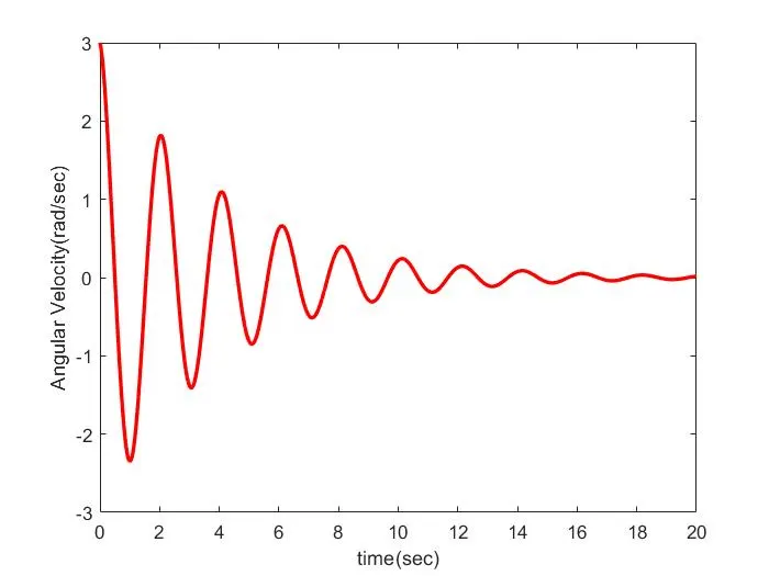
6. The graph of angular velocity v/s time is plotted.
7. The labels for Co-ordinate axes are given using : xlabel('time(sec)'); and ylabel('displacement(rad)');.Here the text enclosed within the single quotes will be displayed as label for the co-ordinate axes.
8. figure(1) command is used to create a seperate window for the graph plotted.
9. The above steps from 2 to 7 are repeated for next graph also,But only the 'y' Co-ordinate changes to results(:,2) (All rows of 2nd column in the results matrix).Therefore the graph is plotted between the time and angular velocity.
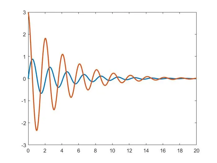
10. Similarly the combined plot is drawn by considering the complete results matrix.The command is : plot(t,results,'linewidth',2);

OUTPUTS :

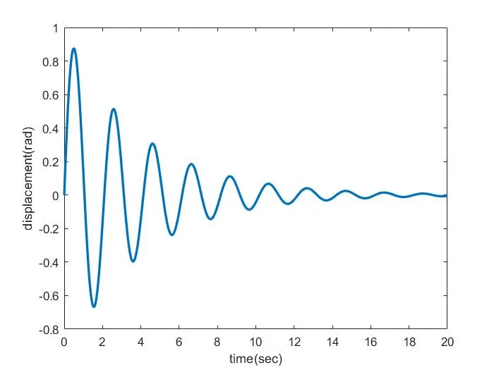
PLOT OF ANGULAR DISPLACEMENT(`theta`) V/S TIME (Sec):

PLOT OF ANGULAR VELOCITY(`omega`) V/S TIME(Sec):

COMBINED PLOT:

ANIMATION OF THE SIMPLE PENDULUM OSCILLATION:

This is the animation of simple pendulum.

ERRORS OCCURED :

IMPROPER SCALING OF AXES CO-ORDINATES:

The command used to set up the ranges for axes is :axis([-1,1,-2,2]);

Here the first two values indicates the range for x-axis and the second two parameters indicate the ranges of y-axis.Here the scaling for the x-axis differs from y-axis.Due to this,the animation would look differently.The animation will look as follows:

Here the length of the string seems to be extensible because the scaling of x-axis is changed compared to y-axis.

CORRECTION :This error can be corrected by using the same scaling range for x and y axes respectively.Therefore the command should be written as : axis([-2,2,-2,2]);

CONCLUSION :

The Projects thus explains the method of solving Differential Equations using ode45 solver and animation of the simple pendulum is done along with recquired plots.

FURTHER IMPROVEMENTS :

The project can be further extended to various real life problems that include Differential Equations.