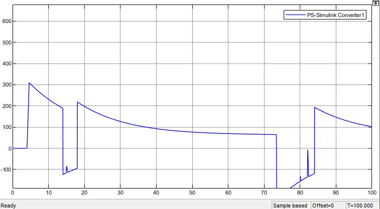
MATLAB model of an electric rickshaw
Create a detailed MATLAB model of an electric rickshaw (three wheel passenger vehicle).
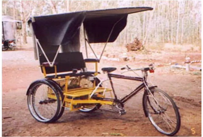
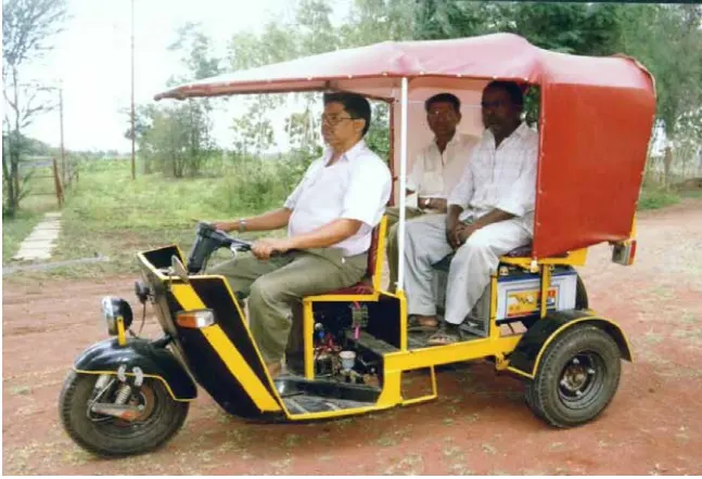
Ans:E-rickshaw development started in the global market sometime during World War period, but faded away with time. These were later introduced in China by local and Japanese motor vehicle industries further spreading in areas of Asia.In India development of e-rickshaw started in late 1990s with the aim of improving manual rickshaws. E-rickshaw was developed with motor assisted pedal rickshaw (MAPRA) by Nimbkar Agricultural Research Institute (NARI). ELECSHA (electric rickshaw) 2000 was also developed later on, but there were issues with battery performance and quality, due to
which these could not trend in market. Illustration of these two models is as follows:
In 1999, Mahindra launched its first electric 3-wheeler.19 Around 2010, E-rickshaws gained prominence in various urban and semi urban areas of UP, Bihar, West Bengal and cities of some other states. Delhi NCR also witnessed a rise in number of e-rickshaws during Commonwealth Games20. E-rickshaws were launched in Delhi with the objective to eventually phase out conventional cycle rickshaws; this objective was eventually altered when e-rickshaws were excluded from NMT category and included in Motor Vehicles Act (2014) as last mile connectivity modal option.
As per Motor Vehicles Act 2014 and Motor Vehicles (amendment) , e-rickshaws are defined as ,A special purpose battery operated vehicle having three wheels and intended to provide last mile connectivity for transport of passengers for hire or reward, provided, such vehicle is constructed or adapted to carry not more than four passengers, excluding the driver, and not more than 40kg luggage in total; net power of its motor is not more than 4000 W and maximum speed of the vehicle is not more than twenty-five kilometer per hour.
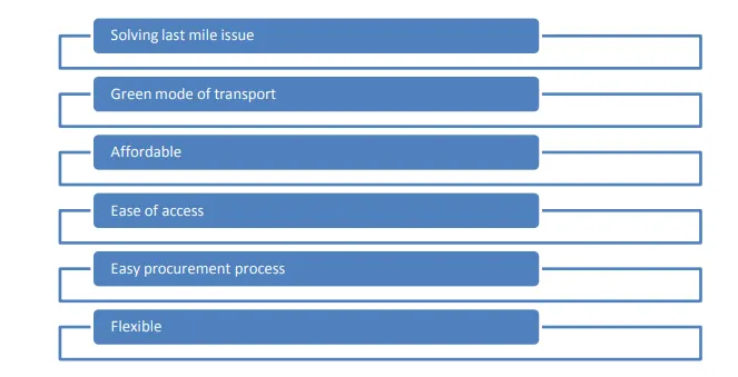
E-Rickshaws are the latest entry in the Indian road and transport system. A flexible, non-polluting and affordable system, they have been playing a significant role in solving the last mile connectivity issue. Due to the absence of rules and norms, they have been largely operating very informally.
While the licensing of E-Rickshaws has been given the nod by the Ministry of Road Transport and Highways, the operation of this system is still ambiguous which has currently led to the ban order by the Delhi High Court. There exists the issue of monitoring and framing the rule book for E-Rickshaws for the safety and security of the commuters using these systems. Policy guidelines are required on whether E-Rickshaws are an Intermediate ParaTransit (IPT) system, who is responsible for the licensing and regulation and how it gets integrated and act as feeder to the public transport. Specific provisions are required to address questions on speed, vehicle specifications,insurance, lane traffic and fare charges. This requires a policy framework to address the concerns of both erickshaw drivers and its counterparts.
Centre for Public Policy Research (CPPR) believes that ERickshaw needs to be integrated into the system at the policy as well as at the infrastructure level and developed as an appropriate feeder system. This demands for a need based assessment and defining of IPT Characteristics in the current public transport system of India. This policy brief aims to develop an approach wherein which systems like erickshaw shall be formally integrated and devised to support the existing systems and enable a sustained transport system.
Benefits of electric rickshaw:
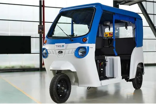
MAHINDRA'S FIRST LOW MAINTENANCE LITHIUM-ION BATTERY POWERED THREE WHEELER:
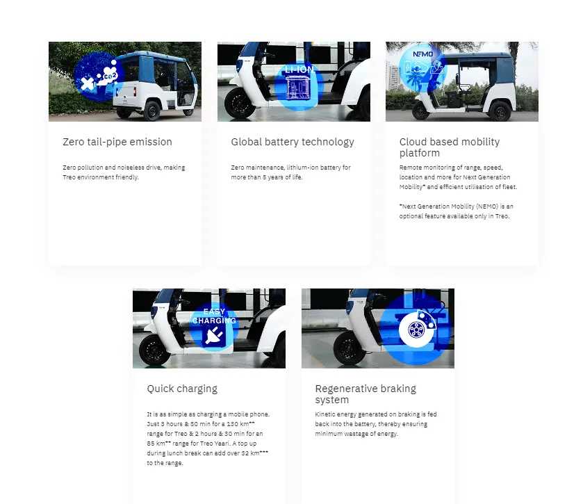
Superior technology:
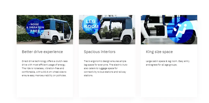
Comfortable ride:
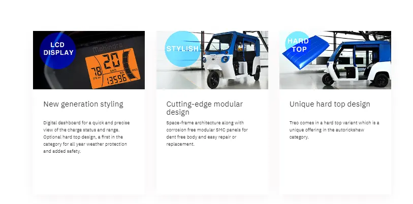
New age style:
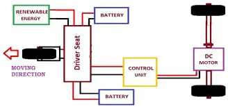
Basic power train of electric rickshaw:
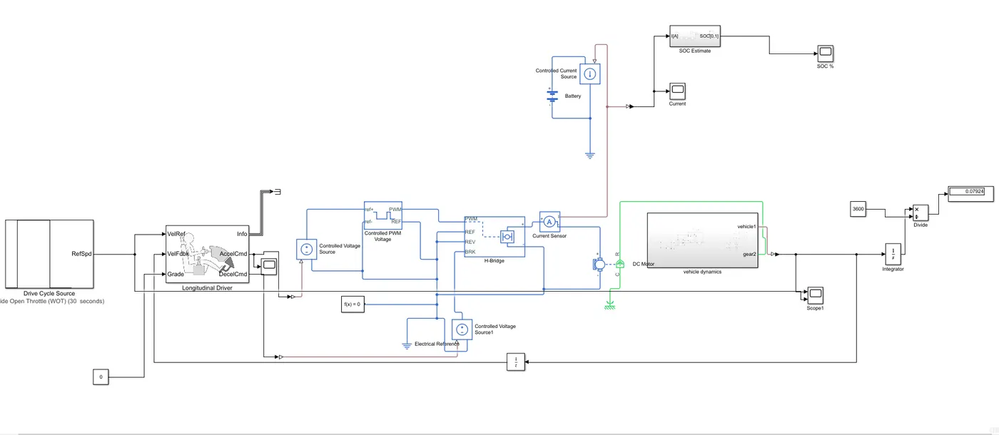
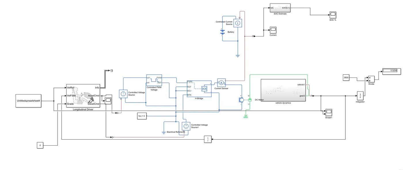
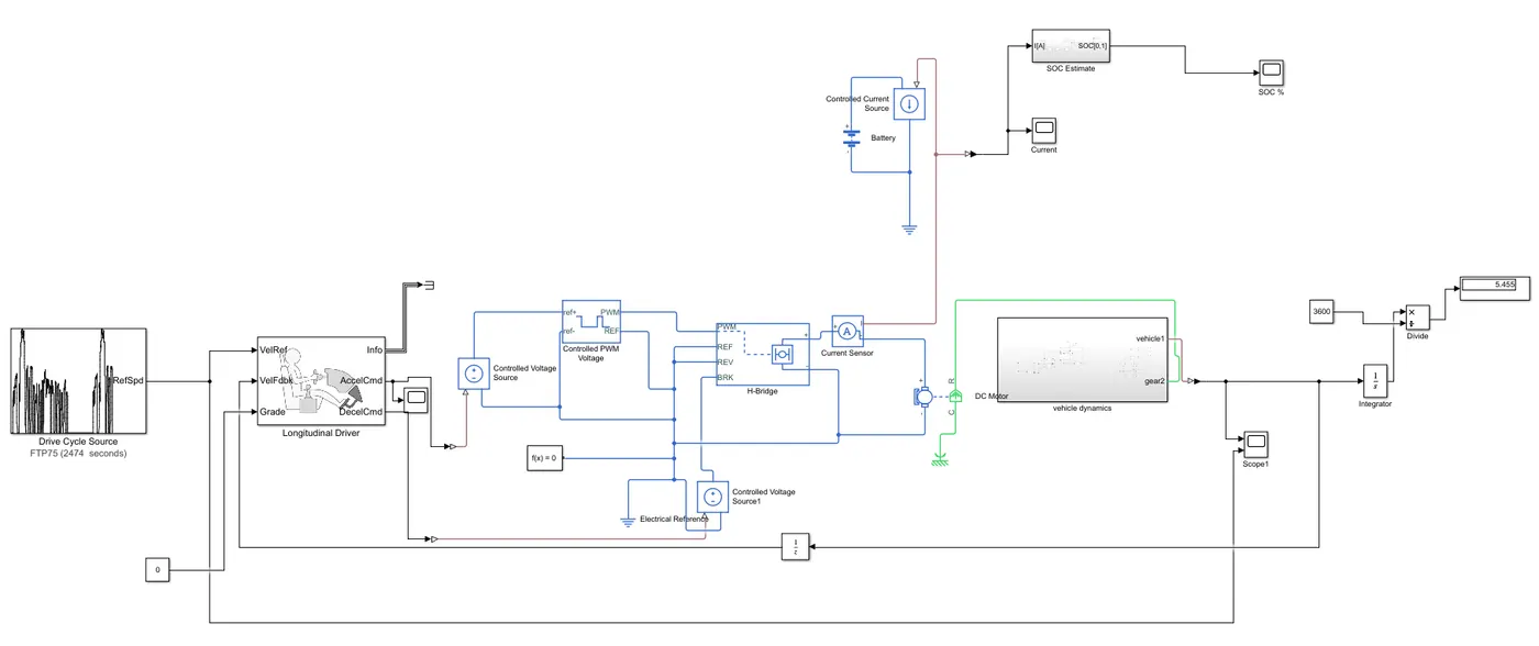
SIMULINK MODEL OF THE ELECTRIC RICKSHAW :
1.Drive cycle:
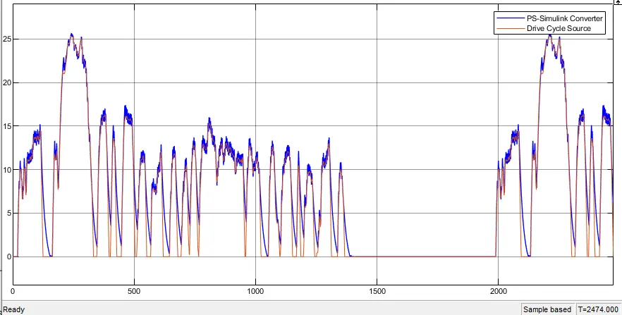
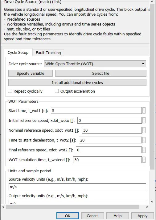
Starting with the drive cycle I have used FTP75 for the operation of the cycle where the stop time is 2474seconds.
The above snap is the FTP75 drive cycle with the max velocity of 26m/s.
Then the drive cycle is connected to Vehicle reference of Longitudinal drive block.
2.Longitudinal driver:
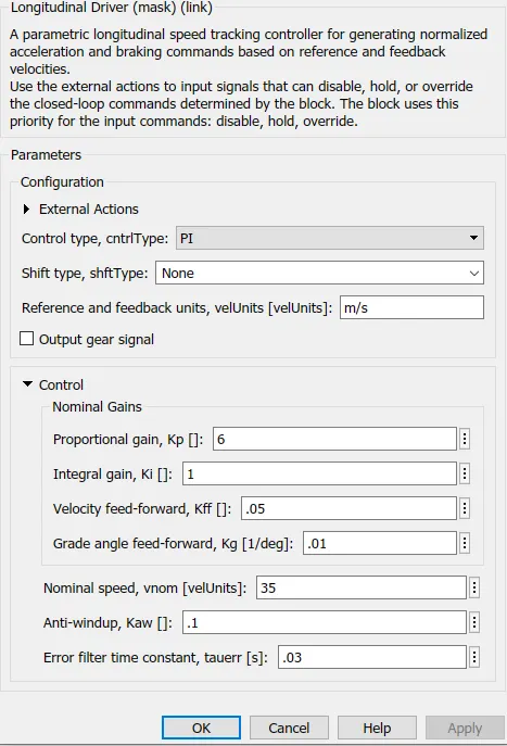
The Longitudinal Driver block implements a longitudinal speed-tracking controller. Based on reference and feedback velocities, the block generates normalized acceleration and braking commands . we can use the block to model the dynamic response of a driver or to generate the commands necessary to track a longitudinal drive cycle.
It consists of six ports they are:
VelREf = vehicle reference
VelFdbk = vehicle feedback
Grade= gradability
info= information which is terminated here.
AccelCmd = acceleration command
DecelCmd = decceleration command
Here speed is taken as feedback through a Smulink PS converter from Vehicle subsyntem and given gradeability for speed calculation integrator blook and a constant is connected with Divide blocks positive and negative terminal respectively. Acceleration command is given to Control Voltage sourcel through a simulink PS Converter.
Parameters considered:
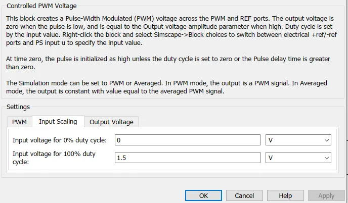
3.Controlled PMW voltage:
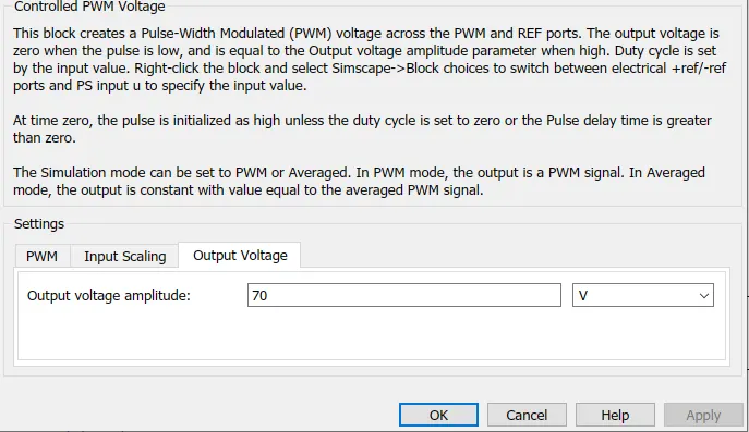
The value of the Output voltage amplitude parameter determines amplitude of the output voltage.
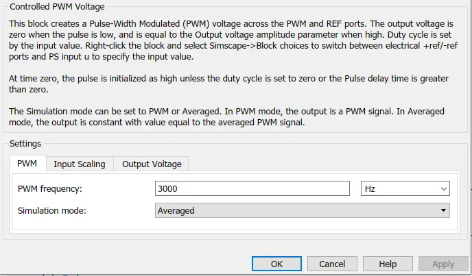
The Controlled PWM Voltage block represents a pulse-width modulated (PWM) voltage source.
-
Electrical input ports — The block calculates the duty cycle based on the reference voltage across its ref+ and ref- ports. This modeling variant is the default.
-
PS input — Specify the duty cycle value directly by using an input physical signal port.
where
-
Vref is the reference voltage across the ref+ and ref- ports.
-
Vmin is the minimum reference voltage.
-
Vmax is the maximum reference voltage
Parameters considered:
4.H-bridge:
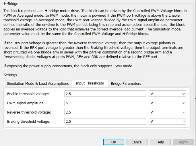
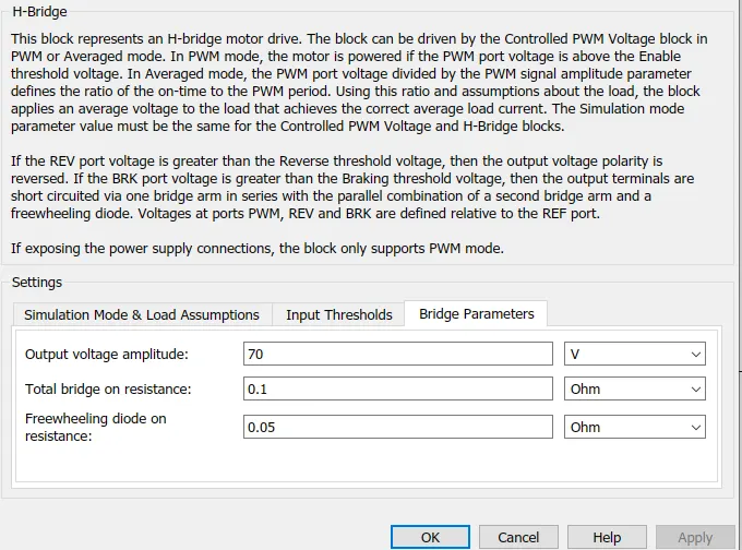
This block represents an H-bridge motor drive. The block can be driven by the Controlled PWM Voltage block in PWM or Averaged mode. In PWM mode, the motor is powered if the PWM port voltage is above the Enable threshold voltage. In Averaged mode, the PWM port voltage divided by the PWM signal amplitude parameter defines the ratio of the on-time to the PWM period. Using this ratio and assumptions about the load, the block applies an average voltage to the load that achieves the correct average load current. The Simulation mode parameter value must be the same for the Controlled PWM Voltage and H-Bridge blocks.Reverse of H-Bridge and both Reference output ot Control PWM voltage and H-bridge is grounded. A solver configuration is connected to the ground reference. Reference output of Control PWM voltage and HBridge is connected.Two output port of HBridge is connected to a DC motors. Also the positive output of bridge is connected to a controlled courent source through a current sensor.
Parameters considered:
5.Battery source:
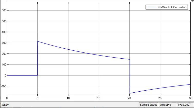
The battery is connected to the H-bridge through the current sensor where the battery is the main power source of the model.
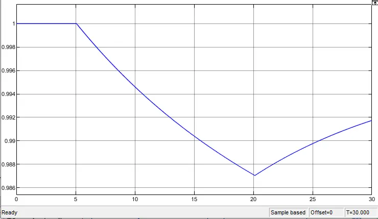
The below model is the complete battery blocks and connections which includes SOC , controlled current sourceand PS simulnk
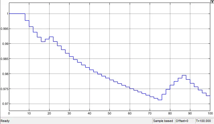
6.SOC estimate block
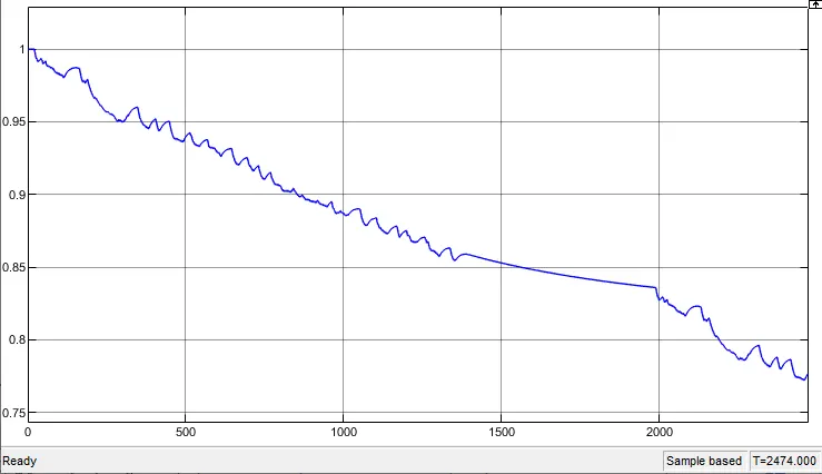
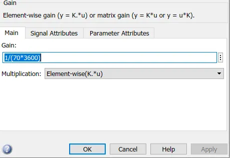
The above subsystem is the SOS estimate block where the rate transition, gain, and discrete time integrator , are connected in series after that this series is added with constant block.This arrangement gives us the SOC.
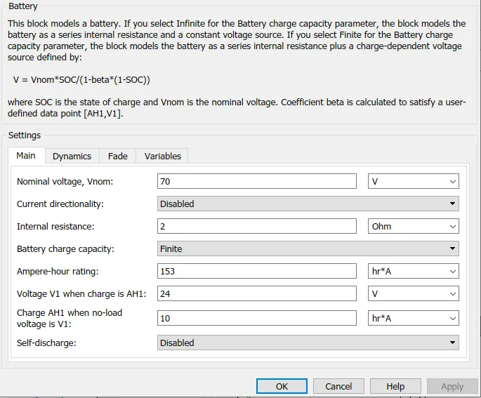
Parameters considered:
7.DC motor:
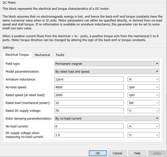
This block represents the electrical and torque characteristics of a DC motor.
When a positive current flows from the electrical + to - ports, a positive torque acts from the mechanical C to R ports. Motor torque direction can be changed by altering the sign of the back-emf or torque constants.
Here the + and - terminals of the dc motor the + and - of the H-bridge respectively.
The mechanical C port is connected to the mechanical rotational reference and R port is connected to the simple gear of the vehicle dynamics block.
Parameters considered:
8.Vehicle dynamics:
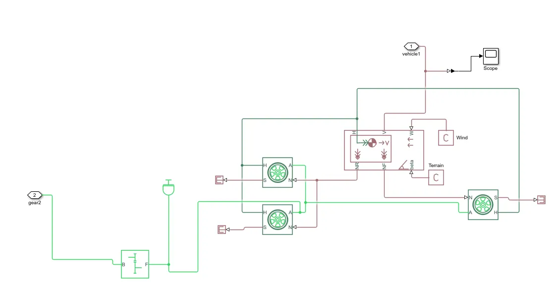
Vehicle dynamic block is a subsystem block which includes vehicle body, gear, terrain, wind, tires, inertia, and PS converter.
Tire:

The above block is Tire with longitudinal behavior given by Magic Formula coefficients.
where H= Hub(Mechanical translational port associated with the wheel hub that transmits the thrust generated by the tire to the remainder of the vehicle).
S= slip (Physical signal output port associated with the relative slip between the tire and road).
a=axle (Mechanical rotational port associated with the axle that the tire sits on).
N=normal force (Physical signal input port associated with the normal force acting on the tire. The normal force is positive if it acts downward on the tire, pressing it against the pavement).
The parameters of the tire is taken as same as default value.
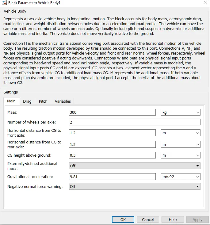
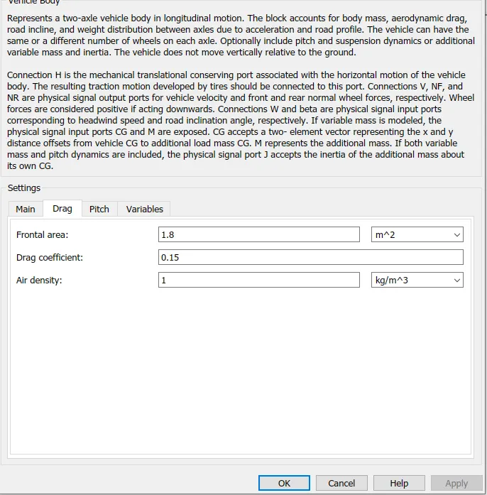
Vehicle body:
The Vehicle Body block represents a two-axle vehicle body in longitudinal motion. The vehicle can have the same or a different number of wheels on each axle. For example, two wheels on the front axle and one wheel on the rear axle. The vehicle wheels are assumed identical in size. The vehicle can also have a center of gravity (CG) that is at or below the plane of travel.
where;
NRNR=rear axle normal force (Physical signal output port for normal force on the rear axle. Wheel forces are considered positive if acting downwards.)
NFNF=front axle normal force (Physical signal output port for normal force on the front axle. Wheel forces are considered positive if acting downwards.)
beta= road incline angle (Physical signal input port for road incline angle.)
WW= wind (Physical signal input port for headwind speed.)
HH= horizontal motion (Conserving port associated with the horizontal motion of the vehicle body. Connect tire traction motion to this port.)
VV=longitudinal velocity ( Physical signal output port for vehicle longitudinal velocity).
Parameters considered:
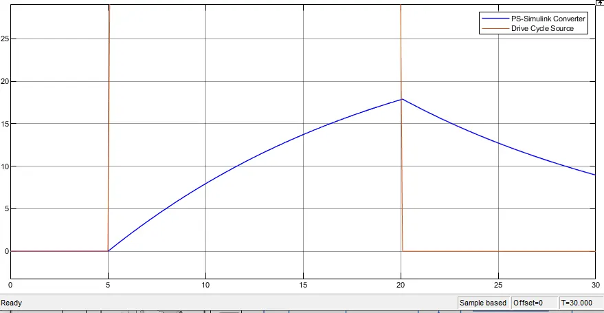
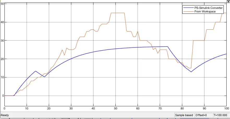
After this, the signal from the velocity port of the subsystem is connected to the scope through the PS converter and for the calculation of distance travelled by the vehicle , velocity port of the subsystem is taken to the integrator block and then it connects divide block as shown in the below figure