1.1.NAVIER STOKES EQUATION

……..(1)

……(2)

……..(3)

………(4)

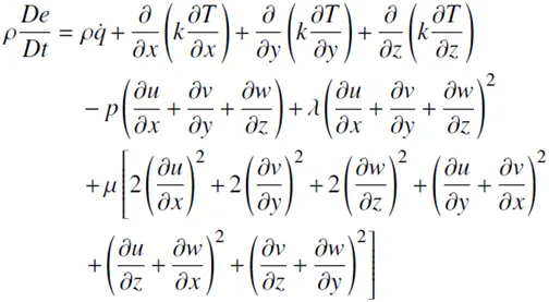
1.2.ENERGY EQUATION

……(5)

2. REYNOLDS DECOMPOSITION

The Reynolds decomposition decomposes the flow variables into mean and fluctuating terms. Let u(x, t) be well defined in a domain Ω ⊂ R^d, d = 1, 2, 3 and for t ∈ [0, tf ] and suppose further that u(x) exists in the sense of the time average. Then the Reynolds decomposition of u(x, t) is,

…………………….(6)

where u′(x, t) is termed the “fluctuating part.” A key observation made earlier is that u(x) is independent of time, implying that any equations derived for computing this quantity must be steady-state. Fig – 1 depicts the temporal behaviors of u and u′.

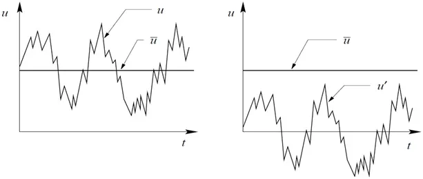
Fig – 1 Plots of parts of Reynolds decomposition

It is important to note that for the type of temporal behavior shown here (probably noisy quasiperiodic, from a dynamical systems point of view) the Reynolds decomposition is likely to provide an inadequate representation. In particular, the mean is seldom attained by the actual signal, and the fluctuating part carries essentially all of the dynamics; in fact, the magnitude of the fluctuations can easily be essentially high as the mean. This is one of the major shortcomings of RANS approaches to turbulence modeling. It is clear from the definition of time average that the Reynolds decomposition possesses the following two properties: u = u , and u′ = 0.

Thus the decomposition of the velocity, pressure, density and temperature can be given as follows :

u = u + u¢ , v = v + v¢ , w =w + w¢ , p = p + p¢ , r=r +r¢ , T=T +T¢..........(7)

3. TIME AVERAGING

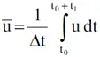
The chosen averaging method takes the mean values at a fix place in space and averaged over a time span that is large enough for the mean values to be independent of it.

……………………………..(8)

The time-averaged values of the fluctuating values are defined to be zero. This is because the fluctuations over have equal positive and negative variations and hence their average is zero.

……………………..(9)

4. DERIVATION OF RANS

Firstly the continuity equation is averaged. If we substitute the expressions for the velocities from Eq – 7 into the continuity equation we get :

………….(10)

The time-average of the Eq – 10 is written as :

………………..(12)

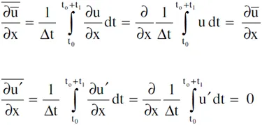
Rules of time-averaging: Time is from t0 to t1

………..…..(13)

……(14)

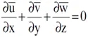
The averaged derivatives of the fluctuations are also zero so that the time-averaged continuity equation is:

…………………………………...(15)

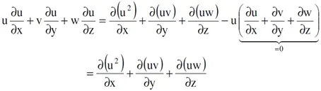
Now the NS equations will be time-averaged. The averaging will be exemplified for the x-

component. Beforehand a small transformation of the advection term from Eq – 1.

…….(16)

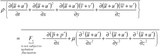
The expressions for the decomposition of the velocities from Eq – 8 are now substituted into the transformed Navier-Stokes equation and a time-average is done:

….(17)

Application of the rules from Eq – 13 and Eq – 14 shows that among others the following terms,

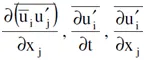
from the equation above can be reduced and the equation can be transformed to :

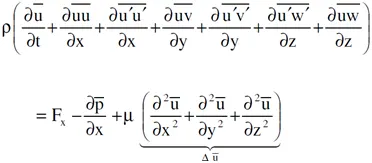…………….(18)

Further small transformations, for example, a repeated application of the product rule and the continuity equation to the advection term, lead to a form of the time-averaged NS equations for all three directions as :

x – component :

……..(19)

y-component :

………(20)

z-component :

……...(21)

In Tensor form :

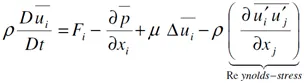…………………(22)

Thus, the time-averaged fields will not be overlined anymore. So for example u stands for the time-averaged velocity component in direction of the x-axis. The Eq – 22 is called the Reynolds Averaged Navier Stokes Equation (RANS).

5. REYNOLDS STRESS

Taking the last two terms in the RHS of the Eq – 22,

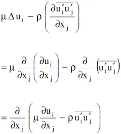………………...(23)

The expression in the brackets above corresponds to the total shear stress :

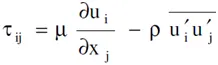……………………….(24)

If we compare to the Navier-Stokes equations, it is conspicuous that besides the viscous part an additional term has been added to the total shear stress.

This term results from the time-average and is generally the dominant part of the total shear stress. Since the term only appears due to the Reynolds average, it is called Reynolds stress or apparent turbulent shear stress. An approximation for the Reynolds stresses has to be done, which sets in relation to the apparent shear stresses with the velocity field of the average flow. Thus, the main aim of turbulent modeling is to capture the Reynolds stress correctly.

TURBULENT VISCOSITY

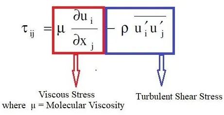
The random eddy motion of groups of particles resembles the random motion of molecules in a gas—colliding with each other after traveling a certain distance and exchanging momentum in the process. Therefore, momentum transport by eddies in turbulent flows is analogous to the molecular momentum diffusion. In many of the simpler turbulence models, turbulent shear stress is expressed in an analogous manner as suggested by the French mathematician Joseph Boussinesq (1842–1929) in 1877 as,

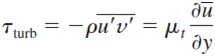
where µt is the eddy viscosity or turbulent viscosity, which accounts for momentum transport by turbulent eddies. Eddy viscosity or turbulent viscosity is the coefficient that relates the average shear stress within a turbulent flow of fluid to the vertical gradient of velocity. The eddy viscosity depends on the fluid density and distance from the walls.

The transfer of momentum caused by turbulent eddies is often modeled with an effective eddy viscosity whereas the momentum transfer caused by molecular diffusion (i.e. friction) is modeled with a molecular viscosity. Eddy viscosity is an imaginary concept and it does not exist as the molecular viscosity which is a well-defined transport coefficient as stated by kinetic theory.