Independent Research Project
Brayton Cycle
AIM : To solve an Air Standard Brayton Cycle (Joule cycle).
OBJECTIVES :
i. To solve an ideal air standard Brayton cycle based on user's input.
ii. To plot it's T-s diagram
THEORY :
The Brayton cycle is a thermodynamic cycle named after George Brayton that describes the workings of a constant-pressure heat engine. The original Brayton engines used a piston compressor and piston expander, but more modern gas turbine engines and airbreathing jet engines also follow the Brayton cycle. Although the cycle is usually run as an open system (and indeed must be run as such if internal combustion is used), it is conventionally assumed for the purposes of thermodynamic analysis that the exhaust gases are reused in the intake, enabling analysis as a closed system.
The Brayton cycle (or Joule cycle) represents the operation of a gas turbine engine. The cycle consists of four processes, as shown in Figure alongside a sketch of an engine:
- a - b Adiabatic, quasi-static (or reversible) compression in the inlet and compressor;
- b - c Constant pressure fuel combustion (idealized as constant pressure heat addition);
- c - d Adiabatic, quasi-static (or reversible) expansion in the turbine and exhaust nozzle, with which we
- take some work out of the air and use it to drive the compressor, and
- take the remaining work out and use it to accelerate fluid for jet propulsion, or to turn a generator for electrical power generation;
- d - a Cool the air at constant pressure back to its initial condition.
#Sketch of the jet engine components and corresponding thermodynamic states.
In practice, real Brayton cycles take one of two forms. An 'open cycle', where the working uid enters and then exits the device. This is the way a jet propulsion cycle works. A closed cycle, which recirculates the working uid. Closed cycles are used, for example, in space power generation.
Closed Brayton cycle Open Brayton Cycle
Work and Efficiency
The objective now is to find the work done, the heat absorbed, and the thermal efficiency of the cycle. Tracing the path shown around the cycle from  -
- - -
- - and back to , the first law gives (writing the equation in terms of a unit mass),

Here  is zero because is a function of state, and any cycle returns the system to its starting state. The net work done is therefore

where  ,
,  are defined as heat received by the system ( is negative). We thus need to evaluate the heat transferred in processes - and - .
For a constant pressure, quasi-static process the heat exchange per unit mass is

We can see this by writing the first law in terms of enthalpy or by remembering the definition of  .
.
The heat exchange can be expressed in terms of enthalpy differences between the relevant states. Treating the working fluid as a perfect gas with constant specific heats, for the heat addition from the combustor,

The heat rejected is, similarly,

The net work per unit mass is given by

The thermal efficiency of the Brayton cycle can now be expressed in terms of the temperatures:

To proceed further, we need to examine the relationships between the different temperatures. We know that points and are on a constant pressure process as are points and , and  ;
;  . The other two legs of the cycle are adiabatic and reversible, so

Therefore 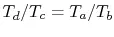 , or, finally,
 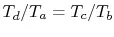 . Using this relation in the expression for thermal efficiency, yields an expression for the thermal efficiency of a Brayton cycle:
 |
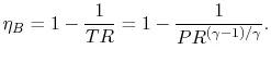
The temperature ratio across the compressor,  . In terms of compressor temperature ratio, and using the relation for an adiabatic reversible process we can write the efficiency in terms of the compressor (and cycle) pressure ratio, which is the parameter commonly used:
 |
Solution Code:-
# A program to solve an air standard cycle for a gas turbine power plant
# Project by Dakshkumar Jadav

import math
import matplotlib.pyplot as plt
import numpy as np

print('Enter the following details:')
print('')
T3 = float(input('Enter inlet temperature at compressor (in degrees C) :n'))
p3 = float(input('Enter inlet pressure at compressor (in MPa) :n'))
ratio = float(input('Enter pressure ratio :n'))
T1 = float(input('Enter maximum temperature (in degrees C) :n'))
eff_t = float(input('Enter turbine efficiency :n'))
eff_c = float(input('Enter compressor efficiency :n'))
gamma = float(input('Enter the value of gamma :n'))

# Inputs
R = 0.287
Cp = R*gamma/(gamma - 1)

# Calculating all state variables
# Converting deg C to K
T1 = T1 + 273.15
T3 = T3 + 273.15
p3 = p3*pow(10,6)

# pressure ratio = p4/p3 = p1/p2
p4 = ratio*p3
p1=p4 # Isobaric Processes
p2=p3

# Ideal gas euation| pV = mRT
v1 = (R*T1)/p1
v3 = (R*T3)/p3

# Adiabatic law | pv^gamma = constant| pressure ratio^(1/gamma) = v3/v4 = v2/v1 || TV^(1-gamma)= constant
v4 = v3*pow((1/ratio),(1/gamma))
T4 = T3*pow((v3/v4),(gamma - 1))

#eff_t(turbine efficiency) = (T4s - T3)/(T4- T3) | T4s is the temperature obtained if the turbine or compressor were completly isentropic
T4s = T3 +eff_t*(T4 - T3)
T2s = T1/pow((p1/p2),(gamma - 1)/(gamma))
T2 = T1 - eff_c*(T1 - T2s)

# Ideal gas law
v2 = (R*T2)/p2
v2s = (R*T2s)/p2
v4s = (R*T4s)/p4

# Calculating work done, heat supplied, thermal efficiency
W_compressor = Cp*(T4 - T3)
W_turbine = Cp*(T1 - T2)
Q_in = Cp*(T1 - T4)
Thermal_eff = (W_turbine- W_compressor)/(Q_in)
print('')
print('At State point 1:')
print('p1 (in Pa) = ', p1)
print('T1 (in K) = ', T1)
print('n')
print('At State point 2:')
print('p2 (in Pa) = ', p2)
print('T2 (in K) = ', T2)
print('n')
print('At State point 3:')
print('p3 (in Pa) = ', p3)
print('T3 (in K) = ', T3)
print('n')
print('At State point 4:')
print('p4 (in Pa) = ', p4)
print('T4 (in K) = ', T4)
print('n')
print('Work consumed by compressor (in kJ/kg) : ' , W_compressor)
print('n')
print('Work done by turbine (in kJ/kg) : ' , W_turbine)
print('n')
print('Heat supplied (in kJ/kg) : ' , Q_in)
print('n')
print('Thermal efficiency of the cycle is: ' , Thermal_eff)
print('n')
int(input('Enter 0 to exit and press Enter:'))
Result:-
# To Solve Air Standard Brayton Cycle and to Plot its T-S Diagram :-
# A program to solve a air standard Brayton cycle and plot T-s diagram
#Program by Dakshkumar Jadav
import math
import matplotlib.pyplot as plt
import numpy as np
import pyromat as pyro

air = pyro.get('ig.air')

# Inputs based on previous program
#inlet pressure at compressor (in MPa)
p1 = 0.1 # in MPa
p1 = p1*10 # 1 MPa = 10 bar

#inlet temperature at compressor (in degrees C)
T1 = 27

#maximum temperature (in degrees C)
T3 = 1000

# Converting deg C to K
T1 = T1 + 273.15
T3 = T3 + 273.15

#pressure ratio
ratio = 6

# Entropy calculation at state 1
s1 = air.s(T1,p1)

# Isentropic Compression
s2 = s1

# pressure ratio = p3/p4 = p2/p1
p2 = p1*ratio

# calculating T2
T2 = air.T_s(s=s1,p=p2)

# Isobaric processes
p4 = p1
p3 = p2

# Entropy calculation at state 3
s3 = air.s(T3,p3)

# Isentropic Expansion
s4 = s3

# calculating T4
T4 = air.T_s(s=s4,p=p4)

# Creating an array of temperature for plotting
T = np.linspace(T2,T3)

# Plotting T-s diagram
plt.figure(1)
plt.plot(air.s(T=T,p=p2),T,linewidth=2,label='Isobaric Heat addition')
T = np.linspace(T1,T4)
plt.plot(air.s(T=T,p=p1),T,linewidth=2,label='Isobaric Heat addition')
plt.plot([s1,s2],[T1,T2],linewidth=2,label='Isentropic Compression')
plt.plot([s3,s4],[T3,T4],linewidth=2,label='Isentropic Expansion')
plt.legend(loc='best')
plt.axis([6, 8.5, 100, 1500])
plt.xlabel('Entropy (kJ/kgK)')
plt.ylabel('Temperature (K)')
plt.grid()
plt.title('T-s diagram of Brayton cycle')
plt.show()
T-S Diagram of Brayton Cycle:-
Method :-
1. At rst necessary modules were imported such as 'math,matplotlib,numpy' were imported for their respective functions. In addition to these one extra module was installed and imported named as 'pyromat'. PYroMat is a Python package for conveniently retrieving the thermodynamic properties of substances from the command line or in scripts.
2. For solving and adding different state variables of gas turbine, user has to input initial conditions such as- temperature and pressure at compressor inlet,maximum temperature which can occur inside plant, pressure ratio, etc.
3. Then the script will solve for these inputs according to their thermodynamic relations and will display in the command window.
4. For plotting T-s diagram, rst thermodyanmic properties of air are imported which is possible through pyromat, and for the inputs provided several other variables such temperature, entropy are calculated. For plotting isobaric curves arrays of temperatures are created and it consists of parts a(2-3) and (1-4). It is returning data at specied intervals. Numpy gives us this feature. Isentropic lines are vertical lines. It consists of coordinates (s1,T1), (s1,T2) and(s3,T3), (s3,T4).
5. For plotting a Graph.
To create a numeric sequence, I used np linespace.
6. legend() , i used legend as in ;- an area describing the elements of the graph.
7. To label the Graph. I used x label, y label for the x-axis and y-axis.
8. To Make visible grid on the graph, i used Plt.grid()
9. Make sure to give the command in the section window.
need to follow the procedure:-
in order to give input i used sublimeREPL
first save the file - then write a code - go to tools - SublimeREPL - Python - select (Python - RUN current file).
after this you can be able to put the inputs. as shown in the below image:-
CONCLUSION :- Python can be a very important tool for mechanical engineers as it has a huge library and a simple syntax which can help you solve complex problems easily and with the help of 'pyromat' module, different types of thermodynamic analysis can also be done easily like Rankine cycle.
References:-
Images and data.
https://web.mit.edu/16.unified/www/SPRING/propulsion/notes/node27.html
#How to install pip and pyromat