Gate Valve Parametric Study

To perform parametric study on gate valve

Objective

For this challenge, you will have to perform a parametric study on the gate valve simulation by setting the opening from 10 % to 80%.

• Obtain the mass flow rates at the outlet for each design point.
• Calculate the flow coefficient and flow factor for each opening and plot the graph.
• Discuss the results of the mass flow rate and flow coefficient.

Parametric study

As you move forward in your design, you can assess the impact that changing certain parameters can have on the design. The parameters can include dimensional parameters. Parametric studies allow you to nominate parameters for evaluation, define the parameter range, specify the design constraints, and analyze the results of each parameter variation.

A parametric study that perturbs design variables in the product design model to explore design alternatives can effectively support product concept designs. A parametric study is simple and easy to perform as long as the mapping between CAD and simulation models has been established. The mapping supports fast simulation model generation for performance analyses.

A parametric study requires the following:

• Design Objective is set to Parametric Dimensions
• Parameters nominated for use in the simulation
• Parameter ranges identified
• Design criteria specified
• Various configurations generated

When you have the configurations generated you can then evaluate your simulation. You can further refine the parameters or design constraints until satisfied with the results.

Once you determine that a configuration satisfies your design needs, you are able to promote that configuration back to the model as a spaceclaim edit. You are prompted whether to make changes.

What is Gate Valve?

A gate valve can be defined as a type of valve that used a gate or wedge type disk and the disk moves perpendicular to flow to start or stop the fluid flow in piping.

A gate valve is the most common type of valve that used in any process plant. It is a linear motion valve used to start or stop fluid flow. In service, these valves are either in fully open or fully closed position. When the gate valve is fully open, the disk of a gate valve is completely removed from the flow. Therefore virtually no resistance to flow. Due to this very little pressure drops when fluid passes through a gate valve.

To achieve proper sealing, when the valve is fully closed, 360° surface contact is required between disk and seats. Gate valves should not be used for regulation or throttling of flow because accurate control is not possible. The high velocity of the flow in the partially open valve may cause erosion of the disc and seating surfaces and also creates vibration and noise.

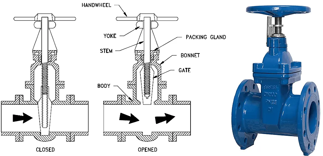
Gate Valve parts

Here you can see the main parts of the gate valve. The disk of a gate valve is also known as a wedge. To learn about each of this part read complete guide of valve parts.

Types of gate valve

There are three ways to classify the gate valve.

1. Types of Disk
   1. Solid taper wedge
   2. Flexible wedge
   3. Split wedge or Parallel disks Valve
2. Types of Body Bonnet Joint
   1. Screwed Bonnet
   2. Bolted-Bonnet
   3. Welded-Bonnet
   4. Pressure-Seal Bonnet
3. Types of Stem movement
   1. Rising Stem or OS & Y Type (Outside Stem and Screw Type)
   2. Non-rising Stem type

Types of gate valve based on body, bonnet connection

Gate Valve applications

• Gate valves are used in almost all fluid services such as air, fuel gas, feedwater, steam, lube oil, hydrocarbon, and all most any services.
• Some special gate valve is used in slurry and powder product also such as knife gate valve

Advantages of Gate Valve

• Gate valve provides good
• Pressure drop during operation is very less.
• Most of the gate valve can be used as bi-directional
• They are suitable for high pressure and temperature application and required less maintenance

Disadvantage of Gate Valve

• It cannot be used to control the flow.
• A gate valve is slow in operation. Opening and closing take times which is good also as it reduces the chance of hammering.
• When partially open it creates vibration and noise.
• Repairs, such as lapping and grinding of seats are more difficult due to limited access.

Geometry preparation for simulation

• In the first step we import the geometry file.
• Then hide the bottom part and go to move option. In the move option select the component part of gate disc. And drag it and gave the value of lift 10 mm and also parametrize it. you can also visulaize it(this thing shown in the below pic). Then uncheck the bottom part.

• In the second step, we extract the fluid volume by using the volume extraction option available in the prepare. Select the inlet, outlet and then hide the bonnet to select the top edge.

• After volume exteraction geometry is

• The flow volume is increased by pulling the pipe outer solid surface from both sides.

• Only the fluid region is analysed, so all unwanted solid components are suppress by using the option suppress from physics. Only the fluid volume is remained acivated.

• Then go to section mode and click on the yz-plane to cut out this section. after creating the plane we observe that fluid volume has not been adapted with the lift. To adapt the fluid volume with the lift, go volume and right click on update volume body in context.

Mesh for lift 10 degree

Mathematical Models

For all types of flows Ansys fluent solves the conservation equations for mass and momentum.

The equation for the mass, momentum can be written as the follows

`frac{partial rho}{partialt}+nabla.(rho bar v)= S_m`

equation (1.1) is the general form of the mass conservation equation and is valid for incompressible and as well as compressible flows. The source Sm">SmSmis the mass added to the continuous from the dispersed phase.

`frac{partial barrho}{partialt}+nabla.(rho bar v barv)= -nablap+nabla .(barbar(tau))+rhobarg+barF`

Where p is the static pressure , `barbar(tau)`the stress tensor, rhobarg and barF are the gravitional body forces and extrenal body force.

Turbulence Models

the k-epsilon realizable model differ from th k-epsilon model in two different ways.

• The k-epsilon realizable model contains an alternative formulation for the turbulent viscosity.
• A modified transport equation for the dissipation rate epsilon, has been derived from an exact equation for the transport of the mean -square vorticity fluctuation.

The term "realizable" mean that the model satisfies the certain mathematical constraints on the reynold stresses, consistent with the physics of turbulent flows. Neither the standard k-epsilon model nor the the RNG k-epsilon realizable.

The modeled transport equations for k and epsilon in the realizable k-epsilon models are.

`frac{partial}{partialt}(rhok)+frac{partial}{partialx_j}(rhoku_j)=frac{partial}{partialx_j}[(mu+frac{mu_t}{sigma_k})frac{partial k}{partialx_j}]+rhobarg+barF+G_k+G_b-rhovarepsilon+Y_M+S_K`

`frac{partial}{partialt}(rhovarepsilon)+frac{partial}{partialx_j}(rhovarepsilonu_j)=frac{partial}{partialx_j}[(mu+frac{mu_t}{sigma_varepsilon})frac{partial varepsilon}{partialx_j}]+rhobarg+barF+G_k+G_b-rhovarepsilon+Y_M+S_K`

Case setup

• Steady state analysis
• Solver type:pressure based
• Velocity formulation:absolute
• Gravity: x=0, y=0, z=-9.81.
• Viscous model: Realizable, K-epsilon model

Near wall treatment : scaleable wall function.

• Material:water

Properties of water: Density=998.2, Viscosity=0.00102

• Cell Zone condition= volume-volume liquid= water
• Boundary Conditions:

• At the inlet boundary we take the pressure inlet type boundary condition. Gauge total pressure = 10 pa.
• At the outlet we take the gauge pressure=0.
• we use the standard initialization.
• After initialization the solution, we have to the set velocity contours.
• Go to solution and then go to definition and set the monitior of mass flow rate at the outlet of the geometry.
• run calculation for 500 iterations.

parametric study setting

• In space claim we make the lift as a input parameter and and mass flow rate as a output parameter.
• in this way we got the result of 10mm lift.
• After getting the first design point result we set the second design point which is 20 mm lift and update.
• similarly we update the design points 30mm to 80mm.

Results

Residuals

Mass Flow Rate

Velocity Contours

As the clearance volume is 10 mm. Due to less clearance volume between the fluid volume and gate disc the values of velocity and mass flow rate are low.

Case-2 (20 degree lift)

Results

Geometry

Residuals

Mass Flow Rate

Velocity Contours

Due to little increase in the lift, we oberve that there is increase in velocity and mass flow rate occur.

Case-3 (30 degree lift)

Results

Geometry

Residuals

Mass Flow Rate

Velocity Contours

Whenever we increase the lift 30 mm we easily that there isincrease of mass flow rate and velocity is occur.

Case-4 (40 degree lift)

Results

Geometry

Residuals

Mass Flow Rate

Velocity Contours

Whenever we increase the lift 30 mm we easily that there is a little increase of mass flow rate and velocity is occur.

Case-5 (50 degree lift)

Results

Geometry

Residuals

Mass Flow Rate

Velocity Contours

Whenever we increase the lift 50 mm we easily that there is a little increase of mass flow rate occur.

Case-6 (60 degree lift)

Results

Geometry

Residuals

Mass Flow Rate

Velocity Contours

Whenever we increase the lift 60 mm we easily that there is a little increase of mass flow rate is occur.

Case-7 (70 degree lift)

Results

Geometry

Residuals

Mass Flow Rate

Velocity Contours

Whenever we increase the lift 70 mm we easily that there is a little increase of mass flow rate is occur.

Case-8 (80 degree lift)

Results

Geometry

Residuals

Mass Flow Rate

Velocity Contours

Whenever we increase the lift 80 mm we easily that there is a little increase of mass flow rate is occur.

Parametric study

In this parametric study we take the lift as a input parameter and mass flow rate as a output parameter.

Flow coefficient and Flow factor

The flow coefficient of a device is a relative measure of its efficiency at allowing fluid flow. It describes the relationship between the pressure drop across an orifice valve or other assembly and the corresponding flow rate.

Mathematically the flow coefficient C_v (or flow-capacity rating of valve) can be expressed as :

`C_v= Qsqrt{frac{SG}{DeltaP}`

where:

Q is the rate of flow (expressed in US gallons per minute),

SG is the specific gravity of the fluid (for water = 1),

ΔP is the pressure drop across the valve (expressed in psi).

In more practical terms, the flow coefficient C_v is the volume (in US gallons) of water at 60 °F that will flow per minute through a valve with a pressure drop of 1 psi across the valve.

The use of the flow coefficient offers a standard method of comparing valve capacities and sizing valves for specific applications that is widely accepted by industry. The general definition of the flow coefficient can be expanded into equations modeling the flow of liquids, gases and steam using the discharge coefficient.

Flow Factor

The metric equivalent flow factor (K_v; commonly used in Europe and Asia) is calculated using metric units :

`K_v= Qsqrt{frac{SG}{DeltaP}`

Where

K_v is the flow factor (expressed in `m^3/h .bar^(-0.5))`).

Q is the flowrate (expressed in cubic metres per hour(`m^3/h`)

SG is the specific gravity of the fluid (for water = 1),

∆P is the differential pressure across the device (expressed in [bar]).

K_v can be calculated using the value of `C_v`

`K_v = 0.865(C_v)`

Density of water 998.2 is`frac{kg}{m^3}`

Pressure drop= 10Pa = 0.0001 bar = 0.00145038

mass flow rate=ρ×volume flow rate

Flow rate = mass flow rate /density of water(`rho`)

Note

The mass flow rate which we got from simulation has unit of `m^3/s`.

Table-1

Lift distance	Mass flow rate	Flow rate	Flow rate(m/h)	Flow rate(US gallon/minute)	Flow coefficient	Flow Factor
10	0.14969876	0.000149969	0.539886901	2.377052414	62.4162765	53.98869013
20	0.24022154	0.000240655	0.866356293	3.814455054	100.1593738	86.63562935
30	0.36133824	0.00036199	1.303162316	5.737655648	150.658479	130.3162316
40	0.47604266	0.000476901	1.716842522	7.559036255	198.4840108	171.6842522
50	0.56315797	0.000564173	2.031022911	8.942332002	234.8063776	203.1022911
60	0.64510575	0.000646269	2.326566662	10.24357303	268.9741643	232.6566662
70	0.71254976	0.000713835	2.569802729	11.31451007	297.0946642	256.9802729
80	0.78781686	0.000789237	2.841252682	12.50966921	328.4769691	284.1252682

Plot of Flow coefficient and Flow factor

In the above graph lift values are represented at x-axis and flow coefficient and flow factor are represented at y-axis. we easily observe that as the lift values are increase flow coefficient and flow factor are increases.

Conclusions

• The parametric study in a gate valve is simulated and analyzed succesfully.
• We easily observed in the results as we increase the lift, there is a gradually increase occur in the mass flow rate.