FSAE Car Project
AIM : To simulate the flow over a formula-1 (FSAE) car and to evaluate downward and drag forces generated.
SIMULATION-SETUP :
- MODEL DESIGN : CATIA V5
- Case setup : CONVERGE CFD STUDIO
- Commanad editor : Cygwin
- Post-processor : Paraview
OBJECTIVE
PHASE-1
- Cleanup the 48 errors
- Flag the front wings, rear wings, tyres, suspension links as separate boundaries
- Create a virtual wind tunnel
- Ground plane reference is provided in the lower end of the tyres. There will be a "flat section" in all the 4 tyres. This refers to the location of the ground plane. You will have to create the ground plane and perfectly merge it with the tyres.
- Run a virtual wind tunnel no-hydro test and a coarse simulation test to prove that you have finished phase 1 correctly.
PHASE-2 - Detailed Setup
ABCD Racing company is looking to perform Aero Simulations for their FSAE vehicle and they have hired you to do the job. The suspension team wants a detailed report on the total downforce on individual components. They have two races in this upcoming season.
Race details are as follows
Race-1
- Racing track conditions - Lot of turns
- Average lap speeds - 45kmph
- 70% turns at 45 degrees
- 20% turns at 80 degrees
- 10% turns at 20 degrees
Race-2
- Racing track conditions - Straights
- Average lap speed - 75kmph
THEORY :
Formula SAE (FSAE) is a student design competition organized by SAE International (previously known as the Society of Automotive Engineers, SAE). The competition was started in 1980 by the SAE student branch at the University of Texas at Austin after a prior asphalt racing competition proved to be unsustainable.
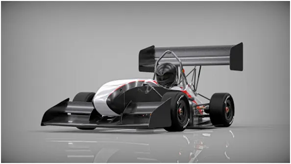
Hence in order to win a race it is very much important that one designs the car aerodynamically good and improves for better performance of it by modifying the car dimensions and weight.
CASE-SETUP :
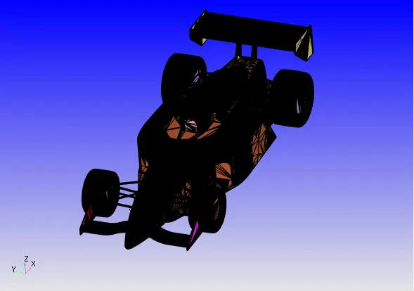
We are going to be setting up the simulation for two different case setup.
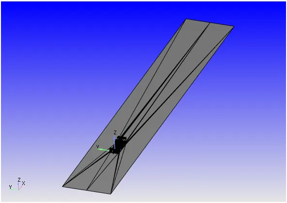
- Straight track : Where car is travelling at an average lap speed of 75 kmph with no turns in the racing track.
2)
- Racing track conditions - Lot of turns
- Average lap speeds - 45kmph
- 70% turns at 45 degrees
- 20% turns at 80 degrees
- 10% turns at 20 degrees
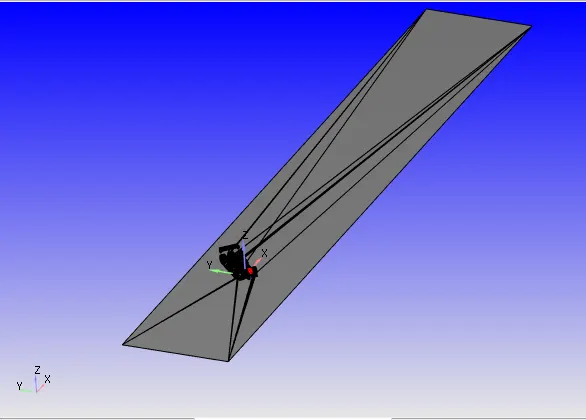
This gives us an average turn of 49.5º
ie,,, (0.7*45+0.2*80+0.1*20) = 49.5º For above mentioned cases the simulation is ran and results are observed.
CASE-SETUP FOR STRAIGHT PATH
CASE-SETUP FOR LOTS OF TURN PATH ( 49.5º )
The geometry was cleaned and all the surface errors were resolved and diagnosis was ran to make sure that there is no surface errors and geometry was ready to setup the simulation.
BOUNDARY FLAGGING :
In order to assign the inlet velocity and all other boundary conditions and to observe the results over particular boundary, the geometry should be flagged into specific boundaries.
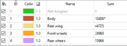
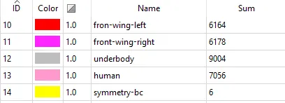
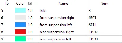
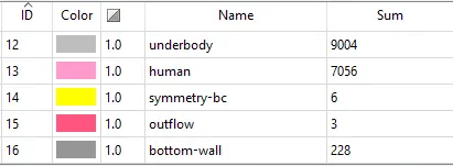
BOUNDARY CONDITIONS :
Inlet
- Inlet velocity of 12.5 m/s for race 1, Re = 2,083,333
- Inlet velocity of 20.833 m/s for race 2, Re = 3,471,667
- Neumann (NE) condition for pressure
Outlet
- Dirichlet (DI) pressure condition at 101325 Pa
- Neumann (NE) velocity condition
Law of Wall
- Law of wall boundary condition for all components of the FSAE car
- Law of wall boundary condition for the bottom wall or the road
Symmetry
- The free space around the car is represented by symmetry boundary condition, since we want the flow properties to be same on both the sides and also for a 2D simulation front and back are just walls.
VIRTUAL WIND TUNNEL :
A virtual wind tunnel was created in order to analyze the flow over the given body. A wind tunnel is an aerodynamic facility to visualize the flow over an external surface. Designing the wind tunnel for any model is a crucial point in any CFD analysis and if the design parameters go wrong, we’ll end up in a wrong simulated answers. Hence setting up a good wind tunnel is a crucial point in any CFD analysis.
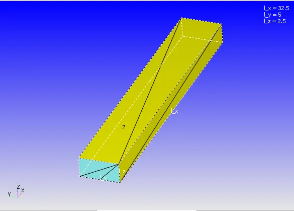
The length of the wind tunnel is 32.5 m is x-direction and width is 2.5 m and has a height of 5 m from the base of the wind tunnel.
SIMULATION-MODE :
The simulation ran was full-hydrodynamic and transient state simulation with solver type being-density based solver.
SIMULATION TIME PARAMETERS :
The entire length of the wind tunnel created is 32.5 m. Say that the flow of 20.83 m/s , starts from inlet and reaches the exit of the wind tunnel, so the time taken by the flow to reach the exit of the tunnel is,
                                             t= dx/v
                                        t=32.5/20.833   =  1.56 sec.
Let us simulate the flow for about 3 to 4 times, therefore total time or end time of the simulation is
1.56* 4 = 6.24 sec 7 sec.
Therefore the simulation starts at 0 sec and ends at 7sec.
Initial time step for the simulation is 1e-7 sec and the minimum time step is also 1e-7 sec and maximum time step of the simulation being 1sec, although the simulation doesn’t reach the maximum time step of 1sec.
Density-based solver is used as it is suitable for both compressible and incompressible flows.
TURBULENCE MODEL :
Standard k−ω model as it is an external flow.
With automatic capturing of wall-function enabled, to capture the growth of boundary layer when a flow interacts with the body. This records the viscous sub-layer in an accurate way
GRID CONTROL (BASE GRID AND FIXED EMBEDDING)
A desired base grid was assigned , where converge predicted around 1.2 million cells analytically. Since we are doing an aerodynamic simulation it is necessary to capture the data accurately around the body that has to be visualized.
Hence fixed embedding of boundary – type was added to capture the data more accurately and to improve the mesh refinement around the body.
If the mesh refinement is good the results obtained for boundary layer will also be an accurate one.
Well, why does the boundary layer develops??
It is due to the effect called “ coanda effect ”. It says that the fluid jet has a tendency to remain attached to the surface (convex) of the body. So when there is a small region of fluid flow, there will be a development of viscosity. Viscosity is the resistance offered by the fluid for it’s flow, the reason for development of viscosity and viscous forces is ‘shear stresses’.
Hence boundary layer is a region of small fluid flow where viscous forces are dominant.
Capturing results in this regions requires an highly refined mesh.
SIMULATION RESULTS :
MESHING AND GRID CONTROL :
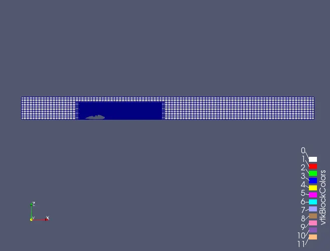
Above figure shows the mesh refinement arounda the car in the virtual wind tunnel. The mesh refined here is a finer mesh and also grid controlling is enabled for higher mesh refinement so that the result captured is
an accurate one.
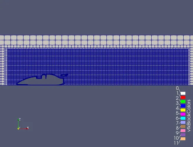
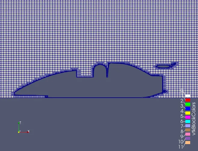
Above figure shows the highly refined mesh around the car, even in small corners the mesh refinement is good to capture the effect of boundary layer.
CELL-COUNT
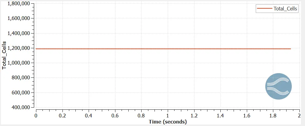
1) FOR STRAIGHT TRACK
2) FOR LOT OF TURNS IN RACE TRACK
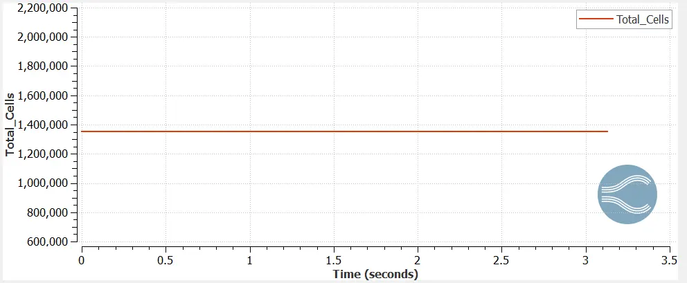
The entire geometry was discretized into finite number of cells or elements. Above plot shows the number of cells or elements created. The total cell-count is constant throughout the simulation.
In first case, since we are doing an external aerodynamic simulation it is important for us to capture the data accurately and in time to time. So the cell count should be higher in order to these functions.
Around 1.2 to 1.35 million cells were created in the simulation.
FORCES ON DIFFRENT COMPONENT OF FSAE CAR :
1) DOWN FORCE ON THE CAR BODY
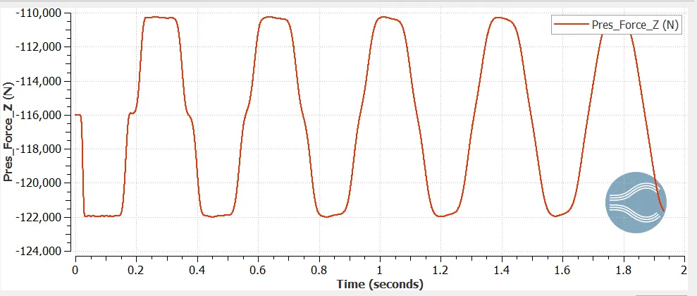
Above plott shows the variation of down force on the car body. With the computational resources limited we can assume the down force cnverges to a value around -118,000 N (-ve sign indicates the force is acting downwards)
Well, why does this down force is important?? It is because it helps the car to stay on the ground rather than to stay in air at such high speed in the races. When the car is moving with higher velocities due to the flow over it the air has the tendency
to lift the car upwards, hence in order to avoid these effects down force plays a major role here.
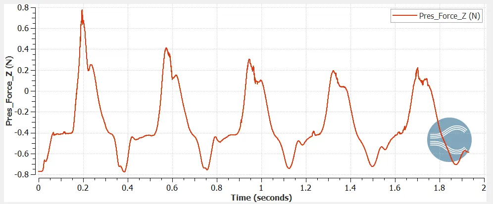
2) DOWN FORCE ON FRONT RIGHT SUSPENSION LINKS :
3) DOWN FORCE ON REAR RIGHT SUSPENSION LINKS :
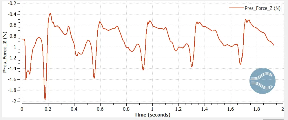
4) DOWN FORCE ON FRONT LEFT SUSPENSION LINKS :
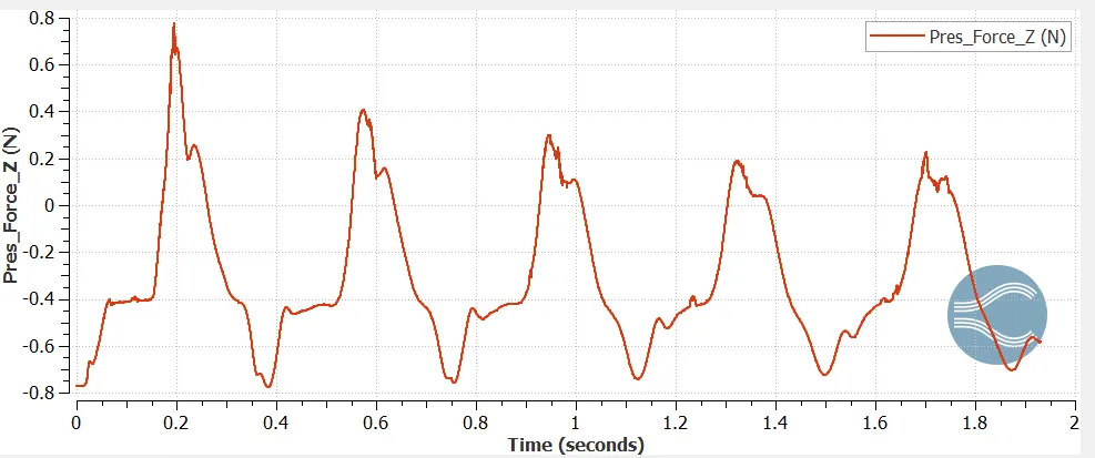
5) DOWN FORCE ON REAR LEFT SUSPENSION LINKS :
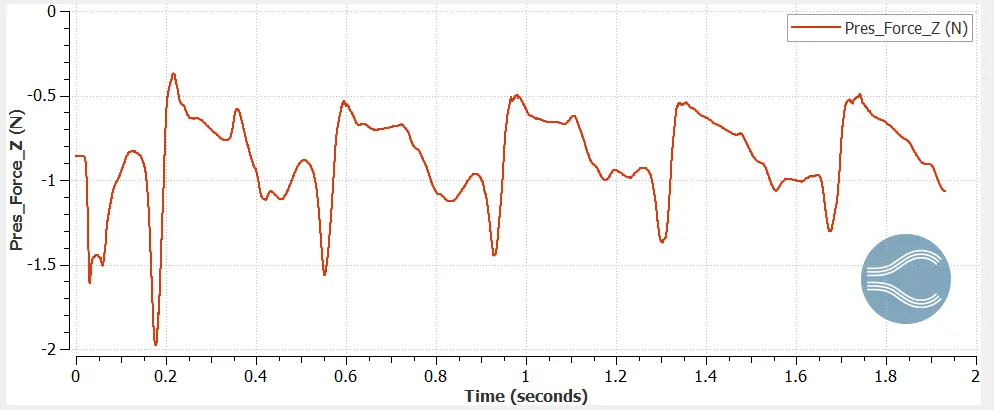
6) DOWN FORCE ON REAR WING :
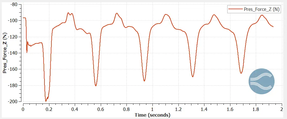
Above plot shows the variation of down force on the rear wing. Rear wing is an important and the most tightly regulated aerodynamiccomponent in a FSAE car (usually called as spoiler).
Well, how does this work??
A rear wing reduces lift. ... In that position, the wind traveling over the top of the wing pushes downward. This downforce then pushes more weight of the car onto the wheels, so they can better bite into the road.
7) DRAG FORCE ON REAR WING :
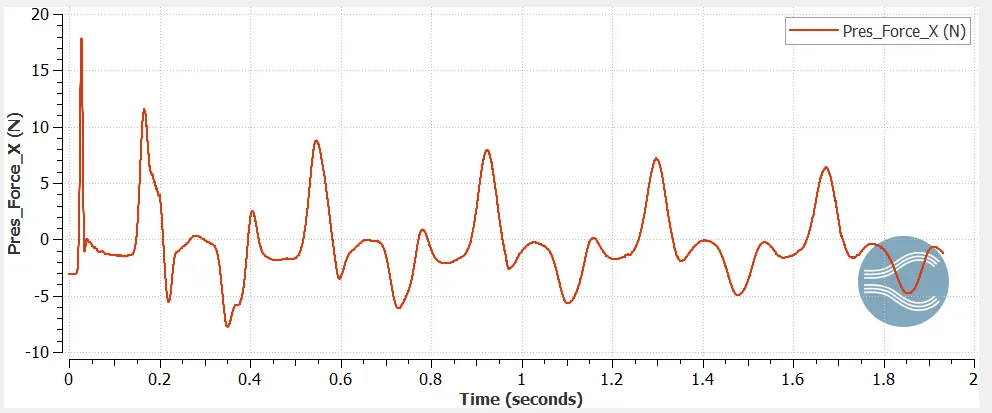
Drag is the resisitance offered by the fluid for it's flow. Usually the rear wing is designed aerodynamically to produce less drag and higher neagtive lift so that the car stays on the ground.
VARIATION OF VELOCITY OVER THE FSAE CAR BODY :
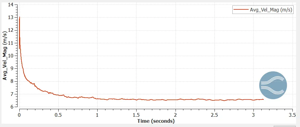
Above plot shows the variation of velocity around the car body. The velocity decreases exponentially and reaches a steady state value of around 7 m/s. The velocity decreases because once the flow
encounters the body it needs to loose it's kinetic energy to flow over it, where there will be increase in pressure rise.
COUNTOUR PLOTS :
CASE-1 : STRAIGTH PATH
1) VELOCITY
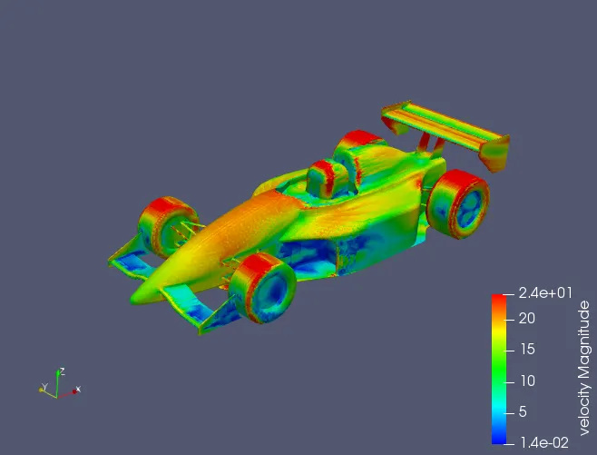
Above figure shows the contour plot of velocity over an FSAE car. When a flow over 20.83 m/s encounters a car or in other words when a car moves at a speed of 20.83 m/s its's velocity over the wheels increases. Above figure
shows it's variation over diffrent components of it.
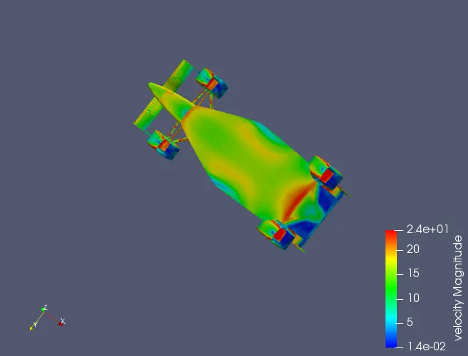
Above figure shows the contour plot of velocity at the botton of an FSAE car.
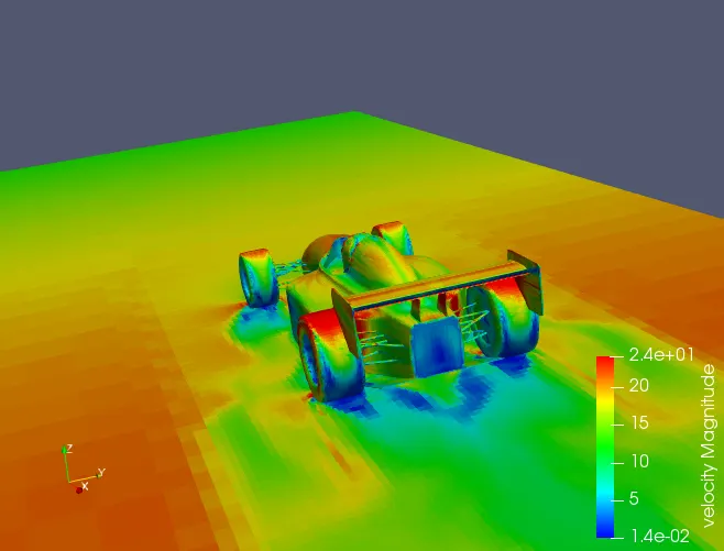
The velocity at the back end of the car is low and also at the contacts where the wheels are touching the ground, velocity is low (about 14 m/s)
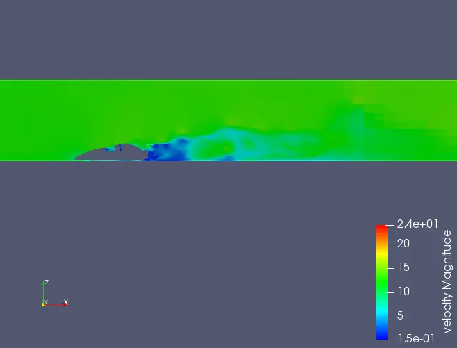
Above plot shows the velocity contour when the flow has just started.
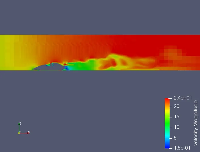
Above velocity contour shows the variation at the time interval of 5 sec since the flow has started.
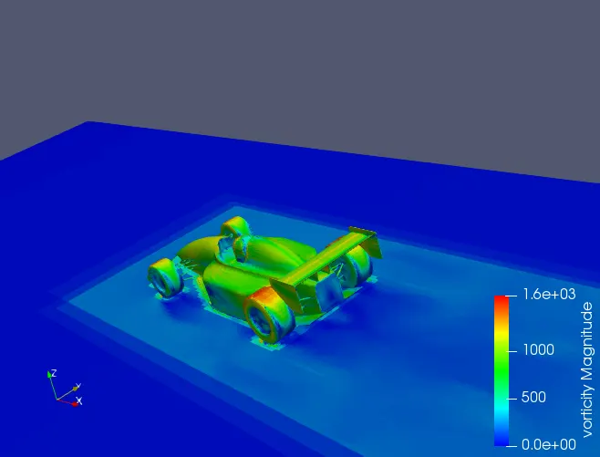
VORTICITY :
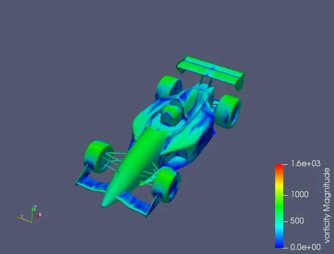
Vorticity is the rate at which the fluid spins on the surface of the body. In fluid mechanics, vorticity is a psuedo vector field that describes the local spinning motion of a continuum near some point (the tendency of something to rotate, as would be seen by an observer located at that point and traveling along with the flow.
CASE 2 : LOT OF TURNS :
1) VELOCITY
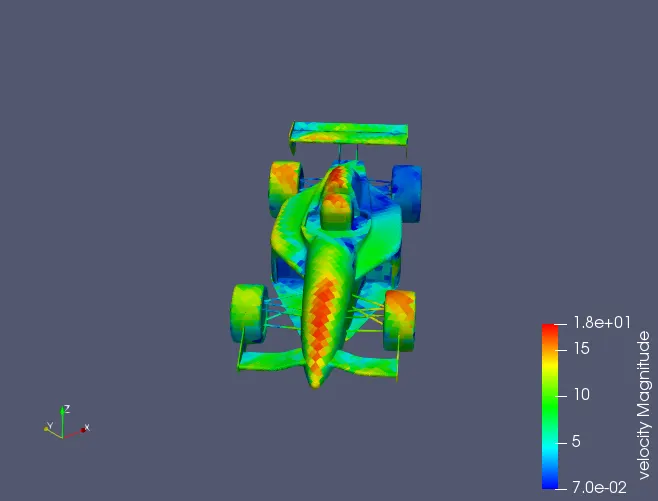
When compared to the previous case here the velocity over the front wheels is much lower and also we can see that the velocity at the rear right wheel is much more lower (around 7 m/s), when the
car moves at a turn of 49.5º
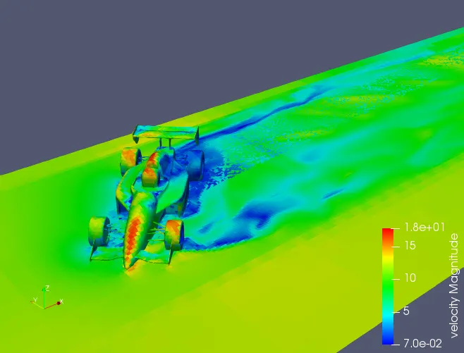
Above contour shows that the velocity is quite a low value at the rear end of the car and the contact surface of the wheels to the ground.
2) PRESSURE
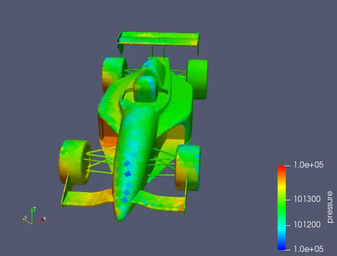
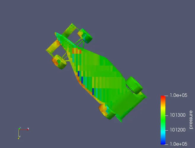
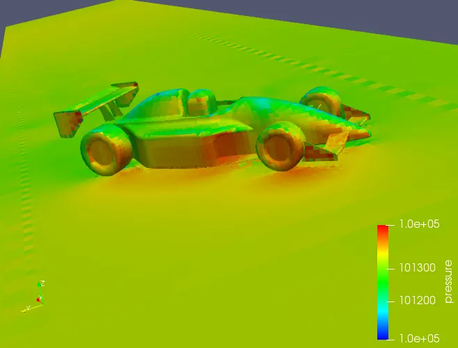
Above figures shows the contour plots of pressure over a FSAE car body when there is flow of 12.5 m/s over it. When a flow encounters the FSAE car body it's pressure increases at the front susoension links which is above the atmospheric pressure.
3) DEPICTION OF FLOW BEHAVIOUR USING STREAM LINES AND GLYPH VECTOR PLOT
Stream lines are the imaginary lines drawns, when a tangent is drawn to it, it gives the magnitude and direction of the velocity at that point. Hence stream tracer was made used to depict
the behaviour of flow over the FSAE car body.
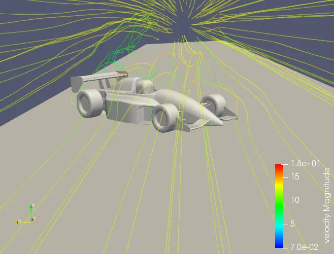
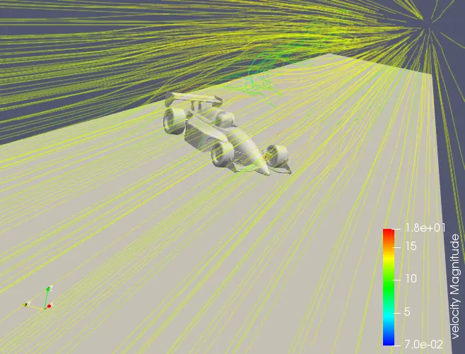
Stream tracer with higher point source and higher resolution.
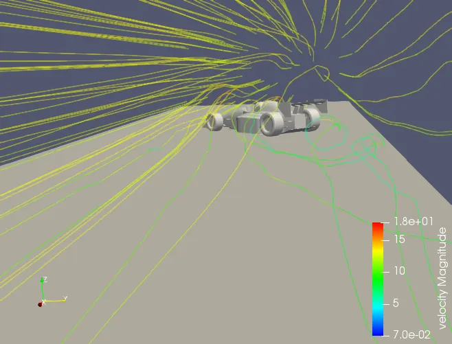
Above figures of stream lines, clearly depicts the behaviour of flow over the body ie,, how the flow is turning or recirculating or slowing down over FSAE car body. At the rear end away from the car
there is recirculation zone and the flow is twisted with lesser velocity.
GLYPH PLOT
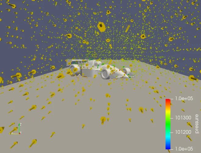
Above figure shows the flow initally when it get's started to move from the inlet to the exit of the wind tunnel.
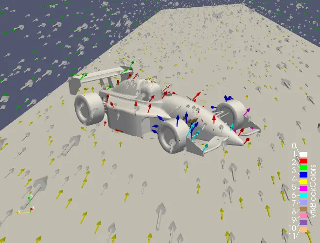
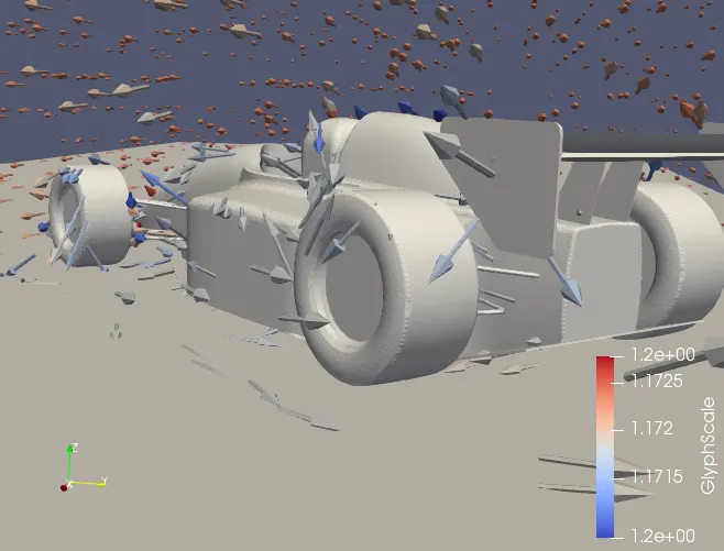
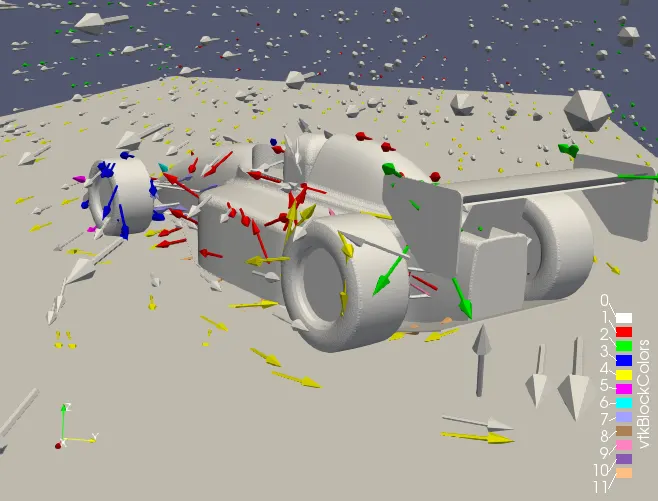
Above figures of vector plot clearly depicts the behaviour of flow around the FSAE car body. The flow is highly chaotic and variation is observed clearly with the help of a glyph plot.
Atthe rea end of the FSAE car the flow is recirculating over the rear wheels and the rear wing and also there is a region just below the rear wing where the flow is getting recirculated and is pointing
towards the rear wing, if this happens some amount of lift will be generated which destroys the tendency of the car to bite or stay on the ground.
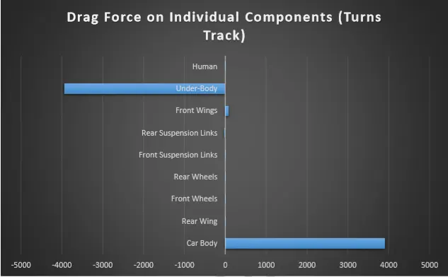
Drag Force on Individual Components (Turns Track)
Down Force on Individual Components (Turns Track)
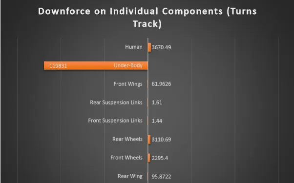
DOWN FORCE-DRAG FORCE (RATIO)
| Component name | Down force (N) | Drag force (N) |
Down force : Drag force (RATIO) |
| Car body | 115982 | 3914.6 | 29.62 |
| Rear wing | 95.362 | 3.6 | 25.20 |
| Front wheels | 2265.4 | 9.1 | 230.50 |
| Rear wheels | 3100.59 | 7.68 | 389.22 |
| Front suspension links | 1.34 | 4.56 | 0.311 |
| Rear suspension links | 1.85 | -30.50 | 0.322 |
| Front wings | 61.96 | 83.5 | 0.752 |
| Under-body | -119831 | -3948.25 | 30.504 |
| Human | 3680.49 | 1.6 | 2353.81 |
ANIMATION LINKS :
CASE - 1 : STRAIGHT PATH
1) VELOCITY CONTOUR
CASE - 2 : LOT OF TURNS
1) VELOCITY CONTOUR
2) PRESSURE CONTOUR
- Conclusion-
After analyzing the data and the result, it was observed that wheels or tires generated a portion of overall drag. To reduce drag on tire, wheels can be covered to make it more aerodynamic. Due to regulation, full covering might not be allowed, but if partial bodywork is permitted, placing converging fairing behind the wheels provides maximum benefit.
According to the result observed in front wing, it did not generate much downforce than needed, thus, the front wing should be designed aerodynamically to increase the overall downforce on the car.
The car body was rotated at an angle of 49.5 degree which is a side slip angle and the tire experiences more load because of turning and high-velocity region in the nose and the air ducts then the low-pressure region in the flow separation region streamline visualization will create drag into rn both combine to produce lift. ( Lot of turns)
The flow over wheels where the top surface of the wheel experiences the higher velocity because the flow over there creates the more the flow front wings where high pressure on top and low pressure on the bottom. The two endplates are fixed to prevent the formation vortices here the vortices are seen at the end so additional drag increases. To reduce the drag is to reduce the airfoil thickness and adding flaps like in an airplanes.
The flow over the rear wing as seen that it creates lift force over the corners by seeing the velocity profiles. This because of the generation vortices and the airfoil in the car wing usually have low aspect ratio and in turn, it creates the drag behind the body and also reduces the angle of attack of free stream air. To improve the lift is to increase airfoil thickness and also increase the height of endplate. The Y plus is uniform throughout the body. The forces on the suspension links are very low and there is a need in change of suspension links.