Flow over a backward-facing step using Converge CFD

Flow over a backward-facing step

Aim: Simulate the flow over a backward-facing step.

Objectives: Run the case for three different base mesh sizes

• dx = dy = dz =2e-3m
• dx = dy = dz =1.5e-3m
• dx = dy = dz =1.0e-3m

• Contents to be shown in the report:
• Show the mesh (i.e surface with edges) for all the 3 base mesh sizes
• Show pressure and velocity contours
• Show the plots of velocity, pressure, mass flow rate and total cell count for all the 3 base mesh sizes
• Also, explain where and why separation is taking place in detail.
• Create an animation.

Theory:

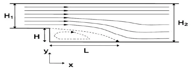
From the above figure, we can see that, at the edge of the step, the fluid boundary layer separates due to the sudden variation in the geometry which causes the fluid to lose some of its kinetic energy which turns the pressure gradient positive causing a free-shear layer to develop inside the original shear layer. The free shear originates due to high velocity on the top of the fluid in comparison to the momentum in the wake of the step. Continuous retardation of the flow turns the wall shear stress negative and the flow reverses and a region of recirculating occurs behind the step which is mostly responsible for the creation of unsteady eddy structure. The flow bubble/recirculation is driven by the low pressure created by the presence of vortices in the separated shear layer. Finally, as the fluid recovers from the sudden expansion, the pressure gradient becomes favorable and the fluid attaches at a position called reattachment point. However, the reattachment(separation) point is an unsteady phenomenon due to the presence of flapping(vortex sheddings). Therefore, to account for the unsteadiness the reattachment point is extended toward the streamwise direction which is known as the reattachment(separation) zone. The skin friction coefficient at the reattachment(separation) zone is zero due to its proportional relationship with the velocity gradient. Ahead of the reattachment zone, the fluid-stream, which has some velocity of the free-stream, propagates forward.

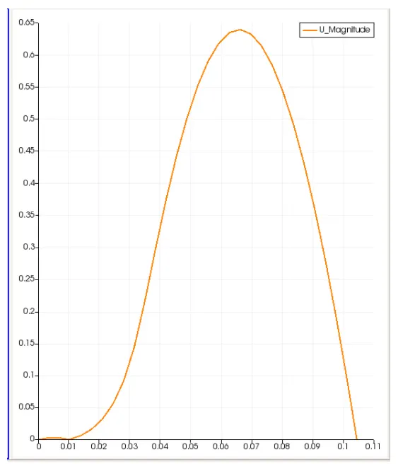
Velocity distribution after flow separation over a horizontal distance

Equations use:

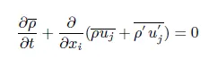
The continuity equation in conservation form represented. The first term in this equation describes the change in density with variation in time and the remaining three terms describes the net flow across the control volume.

Simulation:

The following Simulation tools will be incorporated:

1.Converge studio:- To pre-process the data that needs to simulate the case. It plays an important role in generating important 3d input files only using GUI. It does not run simulation directly, however it generates inputs files which use to run the simulation.

2. Cygwin:- Cygwin is a collection of GNU and open-source tools that provide the functionality similar to Linux distribution on windows.
3. Converge msmpi 3.0:- To run the simulation using these input files in Cygwin in series or in parallel.
4. Post convert:- To convert all the output files which are processed by converge msmpi into the files which will be readable for post-processing in Paraview.
5. Paraview :- To post-processing to obtain the contour, plots, etc. It is an open-source, multi-platform data analysis and visualization software.

Geometry Setup:

Import a Geometry.

Case Setup/Simulation Setup:

MATERIAL:

Gas Simulation:

• Check the Reaction Mechanism.
• Predefined mixture: air

Global Transport Properties

• Turbulent Prandtl number: 0.9
• Turbulent Schmidt number: 0.78

SIMULATION PARAMETER:

Run Parameter:

• Solver: Pressure-based Steady-state
• Simulation Mode: Full Hydrodynamic
• Gas flow Solver: Compressible (as air is working medium)

Simulation Time Parameter:

• End time: 1500 cyc
• Start time: 0cyc
• Initial time step: 1e-06 s
• Minimum time step: 1e-06 s
• Maximum time step: 1 s

Solver Type:

• Pressure based

BOUNDARY:

• Naming: Select faces and name as inlet, outlet, top-bottom wall, front, & back
• Boundary Conditions:
• Inlet:
• Bounady Type: Inflow
• Total Pressure: 110325 Pa
• Specified Boundary condition: Enable Total Pressure
• Species Boundary condition: air

Outlet:

• Boundary type: OUTFLOW
• Pressure: 101325 Pa (Atmospheric pressure)
• Species back flow: Air

Front:

• Boundary type: TWO_D

Back:

• Boundary type: TWO_D

Top-bottom wall:

• Boundary type: wall
• Velocity boundary condition: Law of wall
• Temperature boundary condition: Law of wall
• Turbulent kinetic energy(tke): Zero normal gradient(NE)

REGION & INITIALIZATION:

• Click on Region and Initialization
• Add species: +air
• O2=0.77 & N2=0.3
• Region name as Volumetric Region.

Base grid:

• dx=0.002m; dy=0.002m; dz=0.002m
• dx=0.0015m; dy=0.0015m; dz=0.0015m
• dx=0.0012m; dy=0.0012m; dz=0.0012m

Grid control:

Enable fix embedding to refine the mesh at the wall (as the laminar layer thickness at the wall for Turbulent flow is very less, so to capture the phisics accurately at these low layer region we need to refine the mesh so that we can have a more number of cells there and to get more accurate results)

Click fix embedding-> +Add-> Entry type-Boundary-> Scale of 1(in mm) ->Mode->Permanent.

Post-variable selection:

Output files:

Time interval for writing 3d output data files=100cyc

Time interval for writing restarting output=100cyc

Export input files and Running the Simulation in Cygwin:

Now we have successfully setup the Case and need to export the input files to run the Simulation.

Run the Simulation in Cygwin using parallel processor by disabling Shared memory option.

Post Converting:

Now we need to convert all the output files which are processed by converge msmpi into the files which will be readable for post-processing in Paraview

Paraview:

We need to Post-process the output files to obtain the contour.

Results:

Contour:

For base mesh sizes

• dx = 2e-3m, dy = 2e-3m, dz = 2e-3m
• dx = 1.5e-3m, dy = 1.5e-3m, dz = 1.5e-3m
• dx = 1.2e-3m, dy = 1.2e-3m, dz = 1.2e-3m

Velocity Contour:

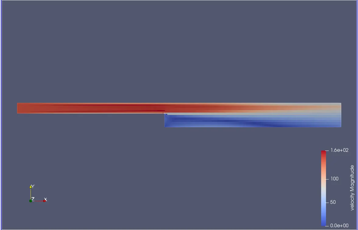
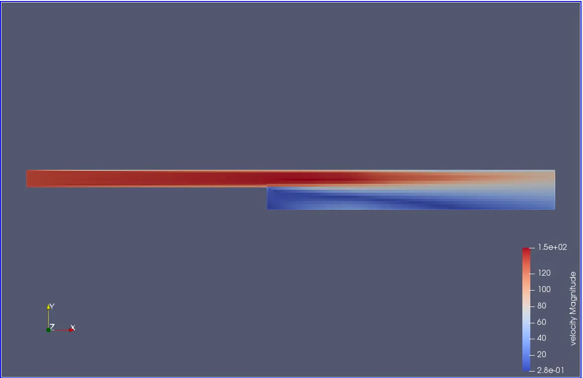
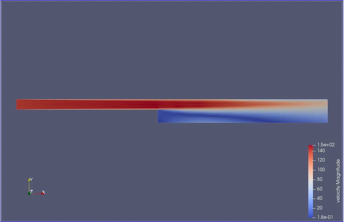
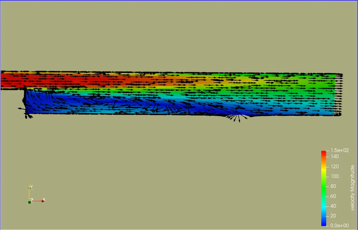
From the above contours, we can see that the velocity is maximum at the inlet and it's decreasing as the flow progresses along x-direction(i.e Space marching). At the stepped section, the velocity is minimum because there is a flow separation, leaving vacuum or low-pressure space in which air is not able to fill properly.

This leads to the formation of vortices due to changing of velocity gradient from positive into a negative value at this point. Hence this point is called a Point of separation. In this point of Separation, the velocity profile du/dy is 0 at the wall. If the adverse pressure gradient acts over a sufficiently extended distance, the deceleration in the flow will be sufficient to change the direction of the flow in the Boundary layer. Hence the Boundary layer develops the Point of Inflection, known as the point of Boundary layer Separation beyond which a circular flow pattern is established as shown in the figure below.

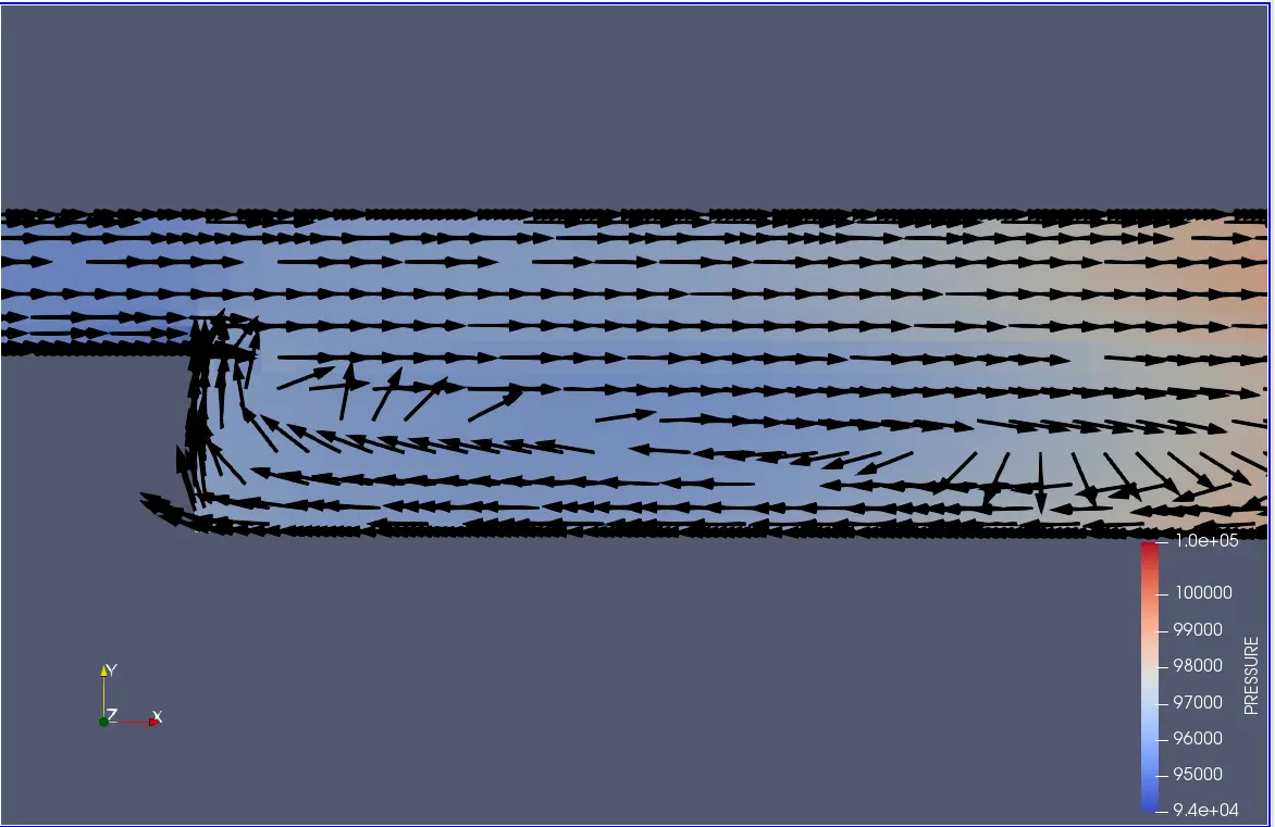
Pressure Contour:

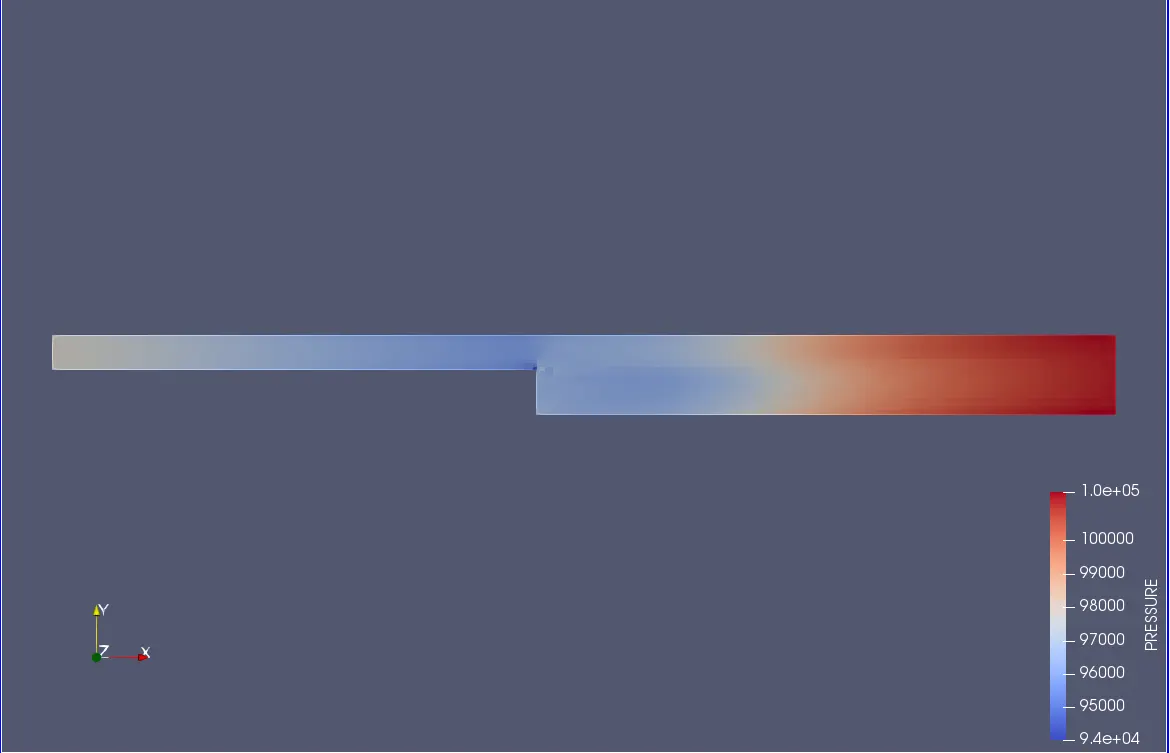
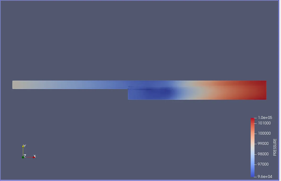
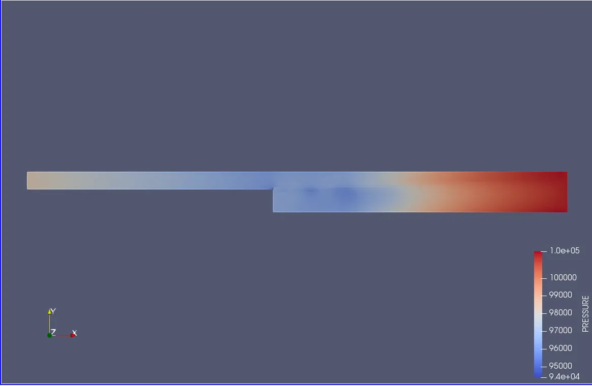
This above pressure contour shows a static pressure only which shows a minimum at the inlet and maximum at the outlet. However, we have applied the Total pressure(static pressure+dynamic pressure) which is maximum than ambient pressure at the inlet.

Show mesh (i.e surface with edges) for the 3 base mesh sizes

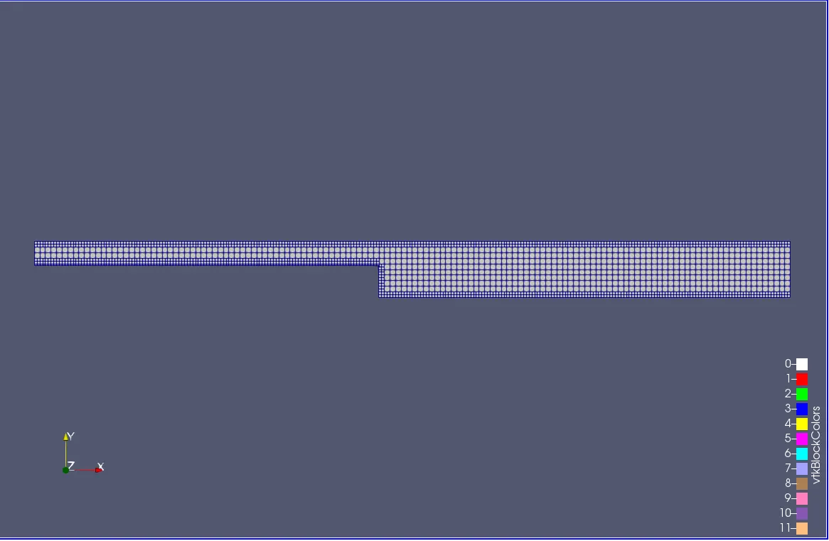
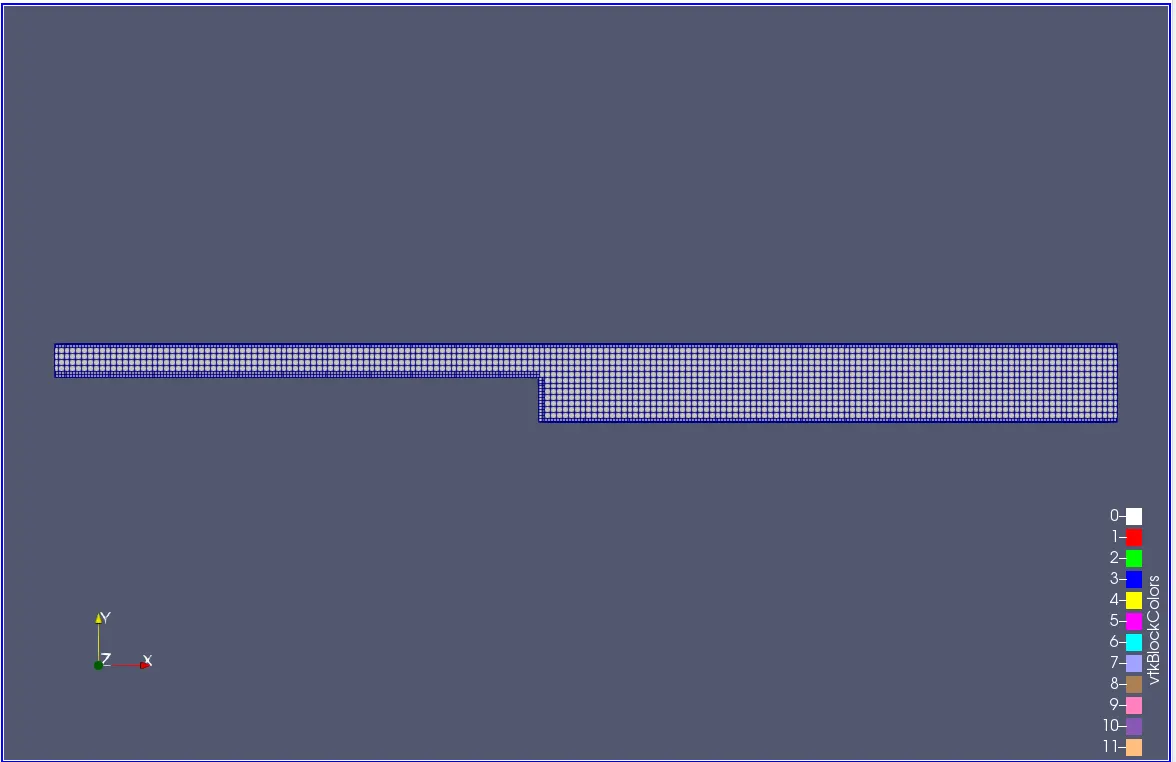
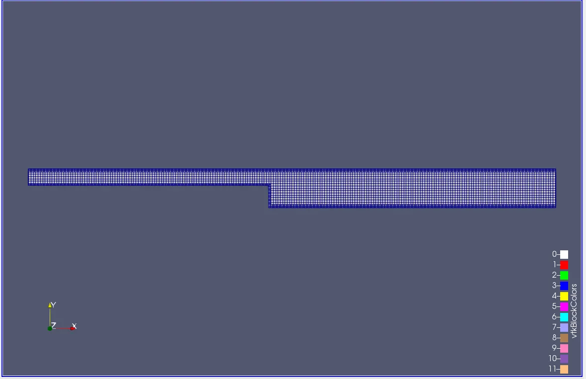
As the size of the Mesh decreases, the cell counts increase. The mesh near the wall is refined as this belongs to the Boundary layer in which we want to capture the physics precisely at the boundary.

Pressure plot:

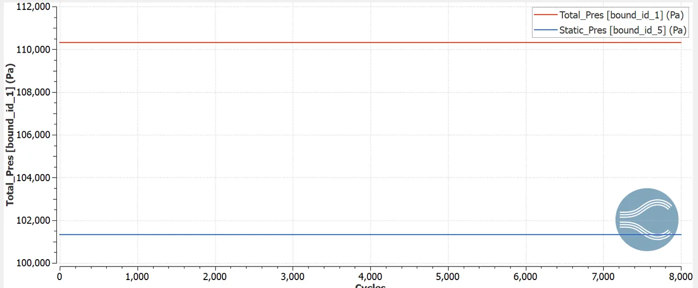
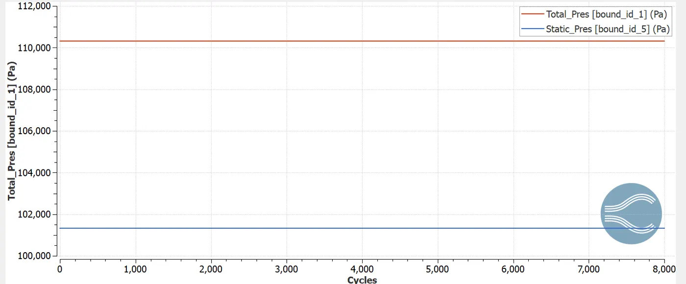
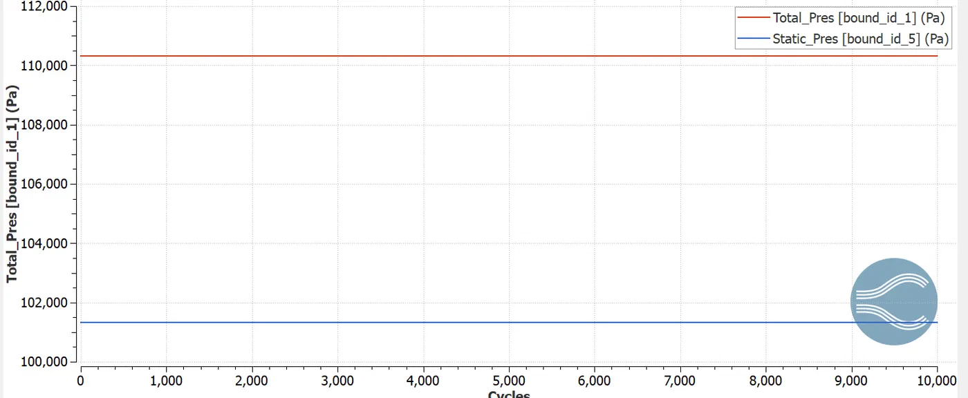
For all the 3 pressure plots of 3 different size meshes the inlet pressure is 110325 Pa and the outlet pressure is 101325 Pa. The number of cycles ran was 8000, 8000, & 10,000 cycles.

Mass flow rate:

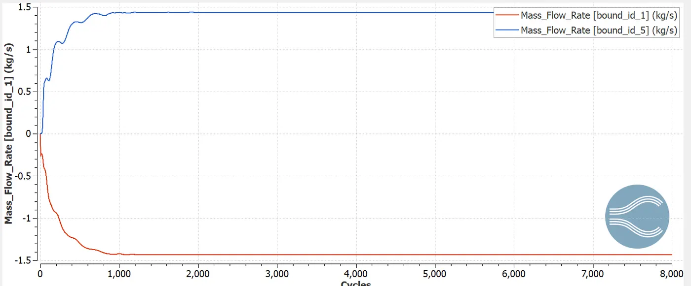
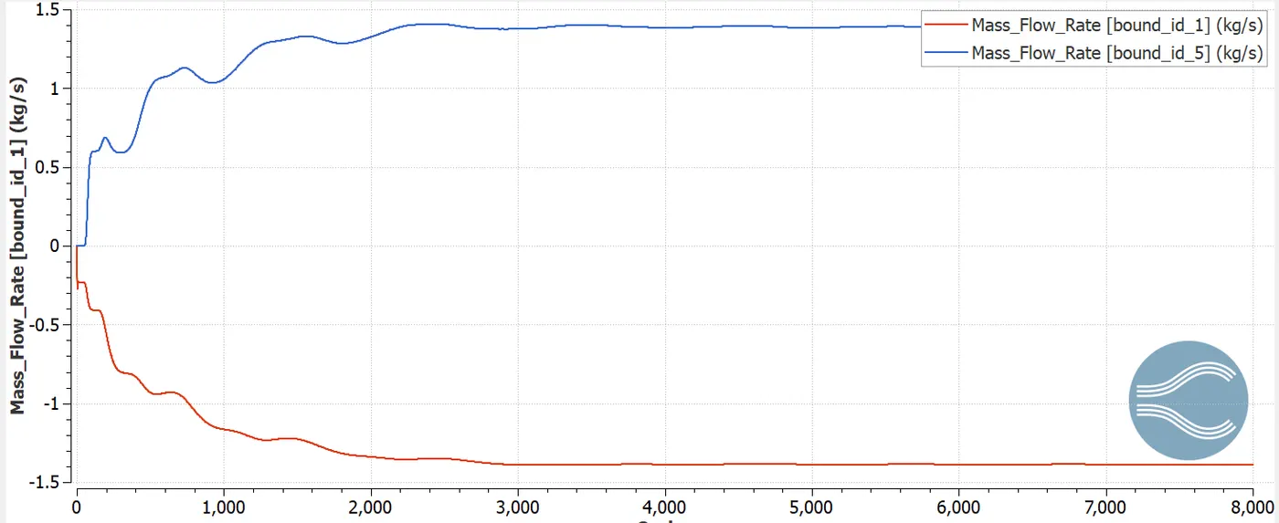
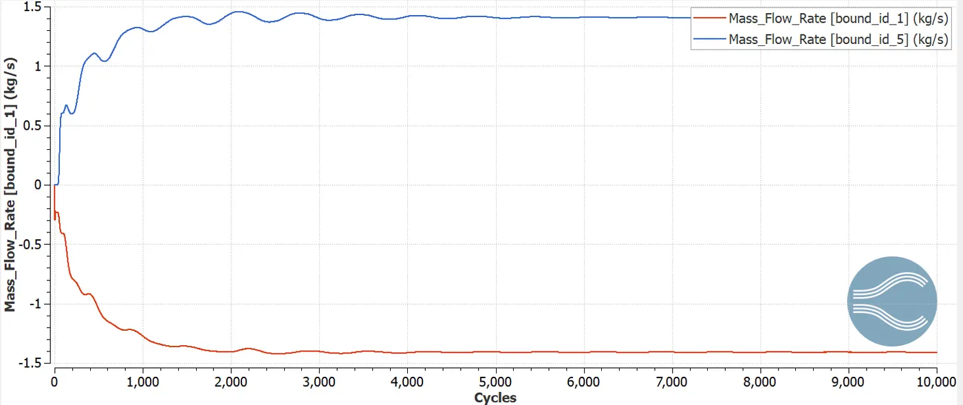
From the above plot, we can see that the solution converges for 3 different sizes of meshes at an increase in the number of cycles, as of 1000, 3000, & 5000 cycles. This is because, as the mesh size decreases the cell counts increase and hence the governing equations need to be solved at more computational cells.

Velocity plot:

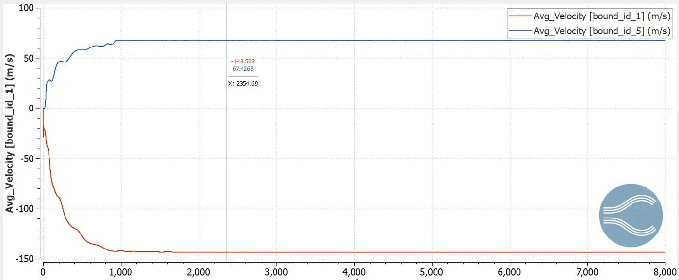
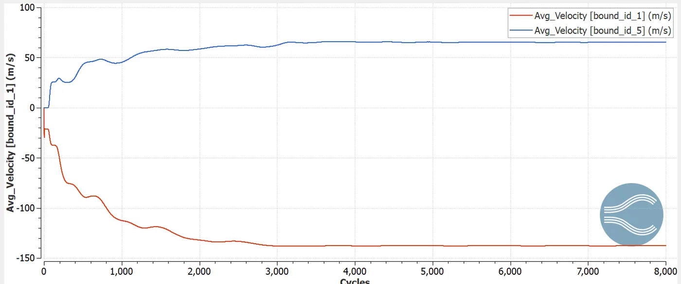
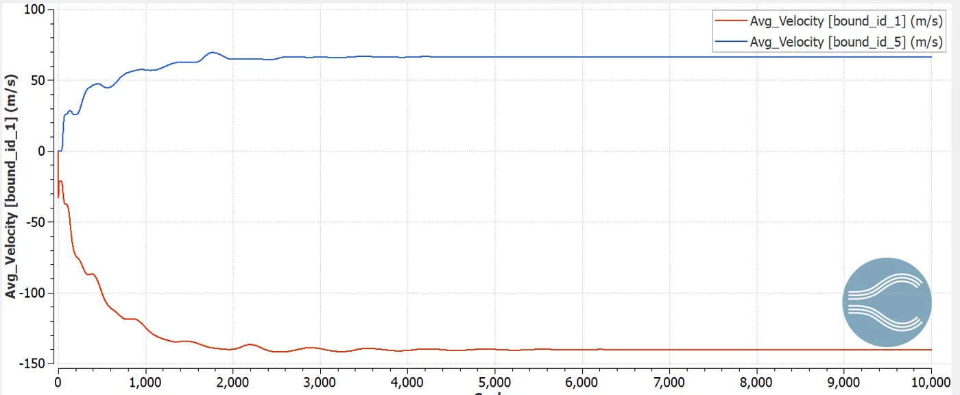
From the above plot, we can see that the solution converges for 3 different sizes of meshes at an increase in the number of cycles, as of 1000, 3000, & 5000 cycles respectively. This is because, as the mesh size decreases the cell counts increase and hence the governing equations need to be solved at more computational cells.

Total cell counts:

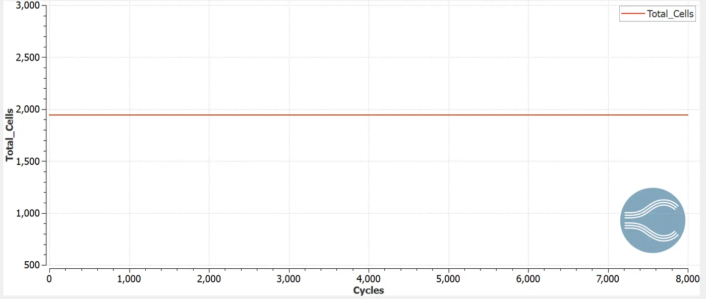
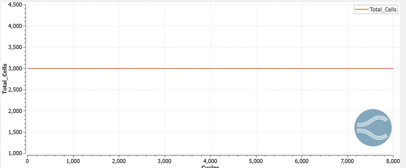
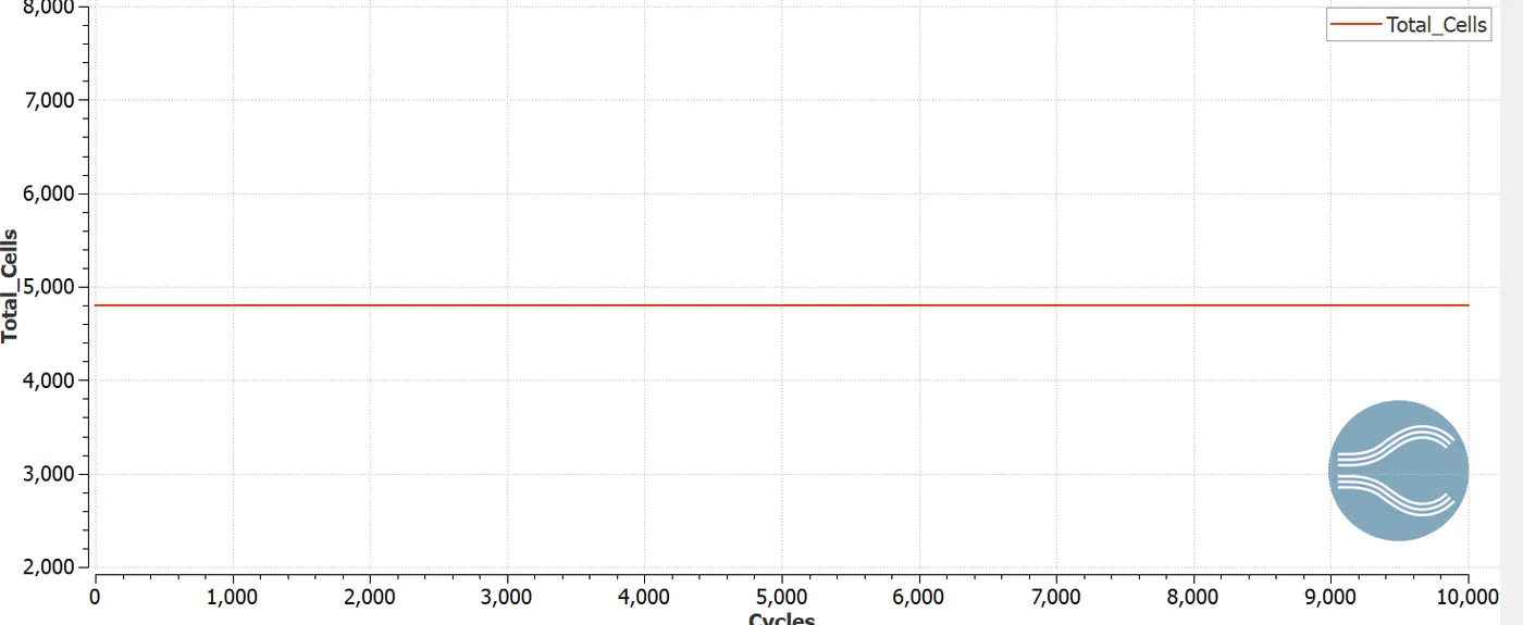
The cell counts increase as 2000, 3000, & 4900 cells (approximately) with a decrease in the mesh size.

Animation:

Conclusion:

• As the mesh size decreases, the number of cycles required for the convergence increases. Hence we get more accurate results for the refined mesh, as the governing equations need to be solved for more grid points.
• The velocity decreases as the flow progresses along x-direction(i.e Space marching). At the stepped section, the velocity is minimum because there is a flow separation, leaving vacuum or low-pressure space in which air is not able to fill properly. This leads to the formation of vortices due to changing of velocity gradient from positive into a negative value at this point. Hence this point is called a Point of separation. In this point of Separation, the velocity profile du/dy is 0 at the wall. If the adverse pressure gradient acts over a sufficiently extended distance, the deceleration in the flow will be sufficient to change the direction of the flow in the Boundary layer. Hence the Boundary layer develops the Point of Inflection, known as the point of Boundary layer Separation beyond which a circular flow pattern is established.