Flow over a backward-facing step

Aim:-

• Set the backward-facing step case setup in the converge.
• Run the base setup with three different base mesh sizes i.e. run 3 simulations and compare the results between all the 3 simulations.
• Plot velocity and pressure contours for all the 3 base mesh.
• Show mesh (i.e surface with edges) for the 3 base mesh size.
• Plot for velocity, pressure, mass flow rate, and total cell count for all 3 base mesh sizes.
• Explain the plots and write a detailed report on the project.
• Also, explain where and why separation is taking place.
• Create animation in Paraview. Explain the development of flow using Paraview

Objective:-

• Create the backward-facing step geometry in the converge using the create option.
• Define the boundary to each surface of the geometry.
• Set normal direction on the inward side of the surfaces.
• In case of setup define the material, simulation parameters, fluid region, boundary condition, no of cycles, grid definition.
• Extract the setup files in the simulation folder.
• Run all the setup file Cygwin.
• Post-process all the results and open in Paraview.
• Show mesh for all 3 mesh bases.
• Plot velocity and pressure contour for all 3 base mesh sizes.
• Plot for velocity, pressure, mass flow rate, and total cell count for all 3 base mesh sizes.
• find out the location of separation and the reason for the separation of flow.
• Create animation in the Paraview to show the development of flow.
• Explain the plots and write a detailed report on the project.

Backward Facing Step Flow:-

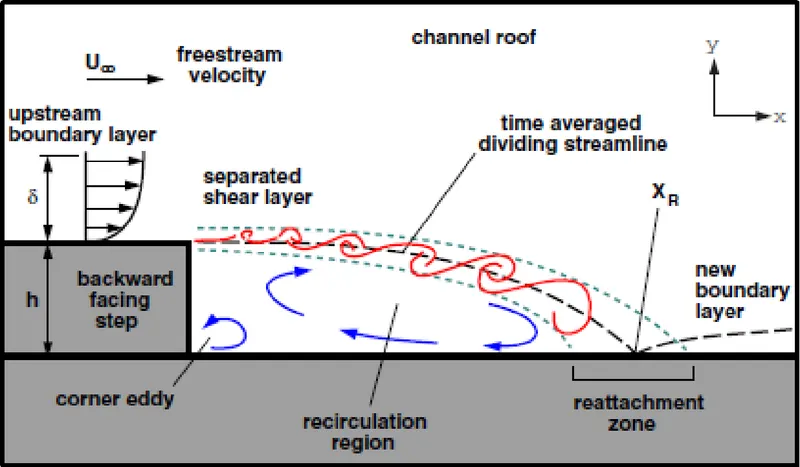
• The examination of simulation on the backward-facing step geometry is very significant for investigating the separation of flow.
• This flow is considered of particular interest because it facilitates the study of the reattachment process by minimizing the effect of the separation process, while for other separating and reattaching flow geometry there may be a stronger interaction between the two.
• The principal flow features of the backward-facing step flow are illustrated in the flowing figure.

• The phenomenon of flow separation is a problem of great importance for fundamental and industrial reasons.
• For instance, it often corresponds to drastic losses in aerodynamic performances of airfoils or automotive vehicles. The backward-facing step is an extreme example of separated flows that occur in aerodynamic devices such as high lift airfoils at large angles of attack.
• In these flows, separation may be created by a strong adverse pressure gradient rather than a geometric perturbation, but the flow topology is similar.
• It is important in heat exchangers and gas turbines also. Since the location of the reattachment zone and its flow structure also determine the local heat and mass transport properties of the flow.
• This geometry has been received attention for half a century. Many researchers considered different aspects of this geometry from the flow pattern point of view and heat transfer.
• In some numerical simulations, the backward-facing step flow problem is a benchmark for validating the computational simulation algorithm.

Geometry Creation:-

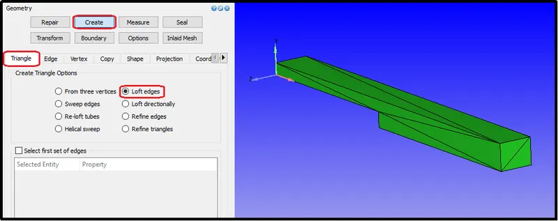
To start the project, as we require a geometry model to simulate, backward-facing step geometry was created by plotting vertex in their exact location.

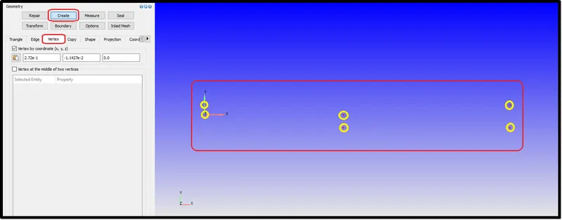
Those points were later used in the creation of the 2d faces by selecting the triangle option in the creat menu. By selecting any three-point we can create a triangle. that way the complete surface was generated with the help of tringles.

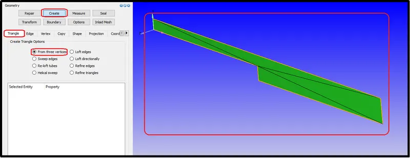
By offset, a command was used to offset that surface so we can create a similar surface at a particular distance along the z-direction.

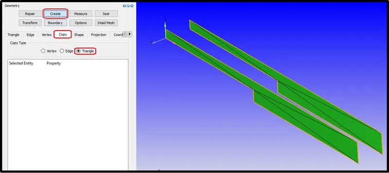
later, the two surfaces were joined using the loft option as illustrated in the below picture.

Boundary Definition:-

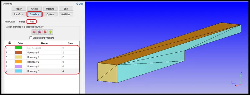
Boundary names were provided to each surface to assign proper boundary conditions to each face of the channel flow model.

Simulation Setup:-

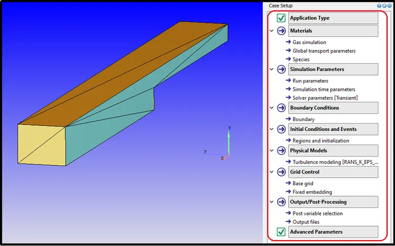
The case setup was created after setting up the geometry and boundary definition.

Application Type:-

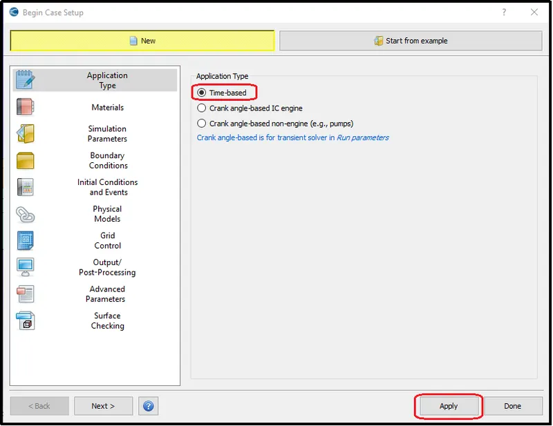
To perform normal steady-state simulation in setup application type we have to select a time-based option.

Material:-

In the material section 'Air' as fluid was considered.

Species:-

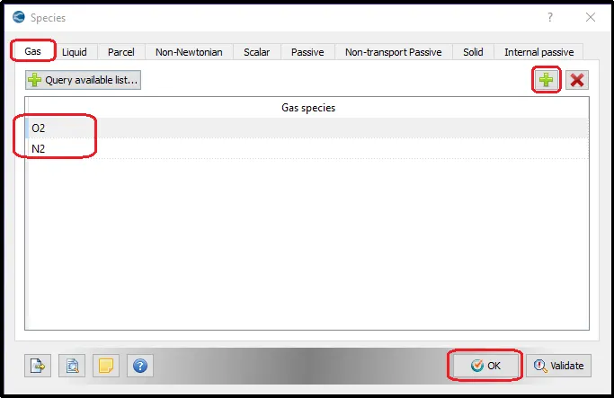
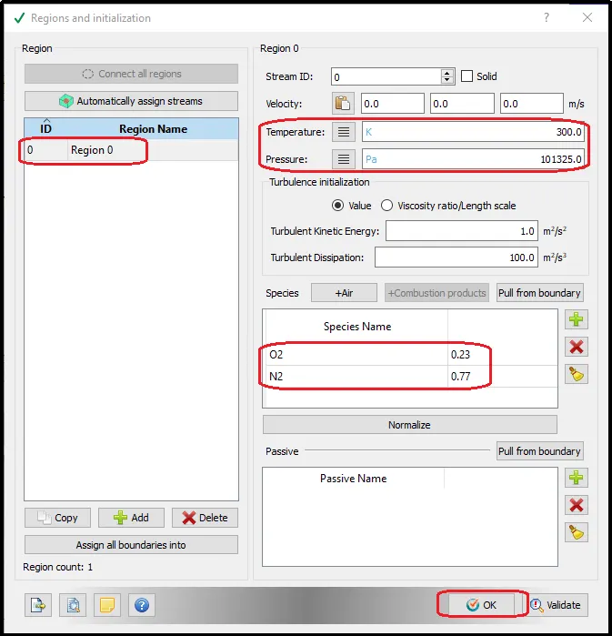
Species were defined as O2 and N2 as air is a mixture of Oxygen and Nitrogen.

Simulation Parameters:-

Run parameters:-

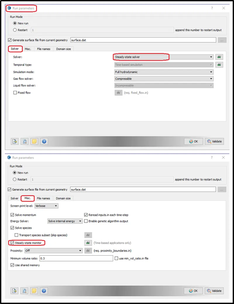
In the run parameter, the solver setup as the steady-state solver is defined. And in misc. Section the steady-state monitor was turned on to monitor the steady-state velocity for convergence of the cycle.

Steady-state monitor:-

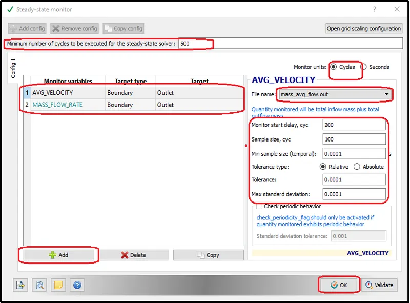
Velocity monitor is set up with proper tolerance to keep track of velocity for convergence of results.

Simulation time parameters:-

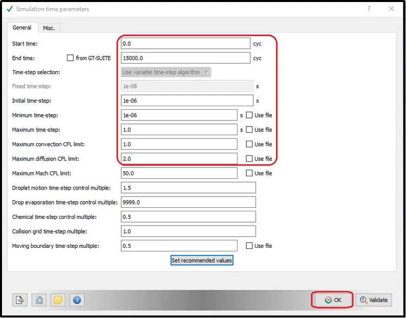
General setting:-

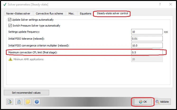
Solver parameters [steady-state]

Steady-state solver control setting:-

Initial PISO convergence criterion multiplier (relaxed): 0.5

Boundary condition:-

Boundary:-

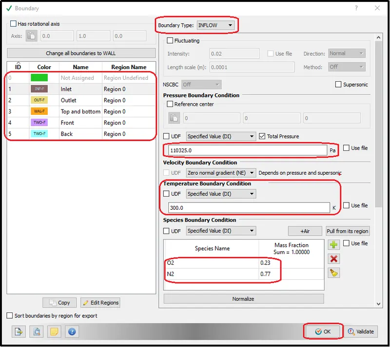
Inlet

For inlet boundary type as inflow selected with 100001Pa pressure and 300k temperature. And air species condition was specified by specifying O2 and N2 percentage as air is a mixture of 0.23% Oxygen and 0.77% nitrogen.

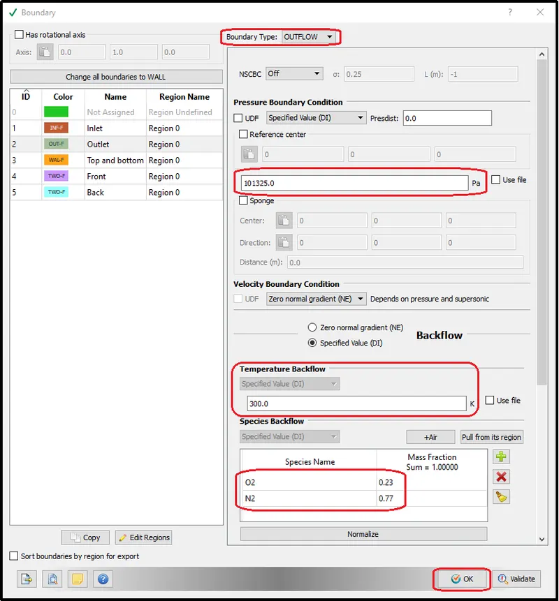
Outlet

At the outlet, boundary type OUTFLOW was selected, with outlet pressure 100000Pa and temperature as 300K. and air species condition was specified the same as an inlet.

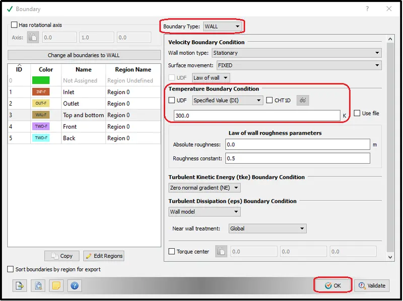
Top and Bottom Wall

Top and Bottom faces were defined as walls with No-slip Condition and 300k temperature.

Side Walls:-

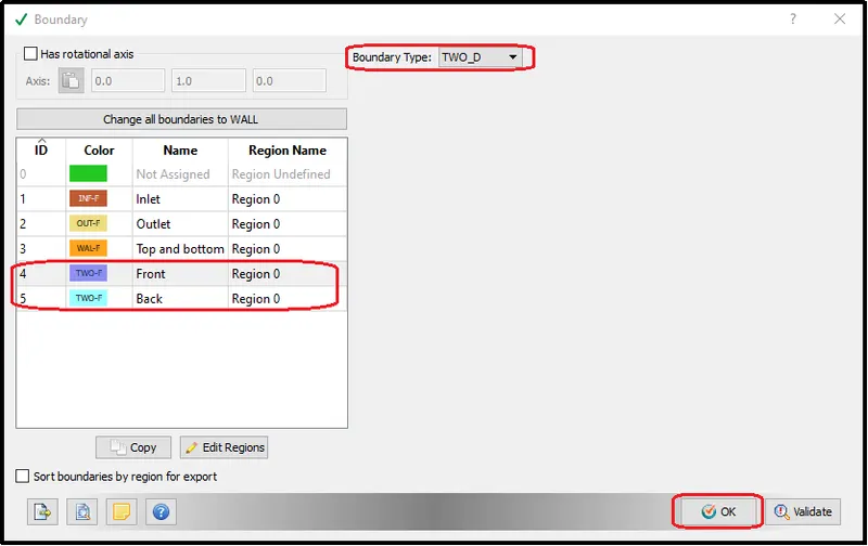
Left side ---> TWO-D

Right side ---> TWO-D

Initial conditions and Events:-

Regions an initialization

The initial fluid region was specified as air with 100000Pa pressure and 300K temperature and named as ‘flow volume’.

Turbulence Model:-

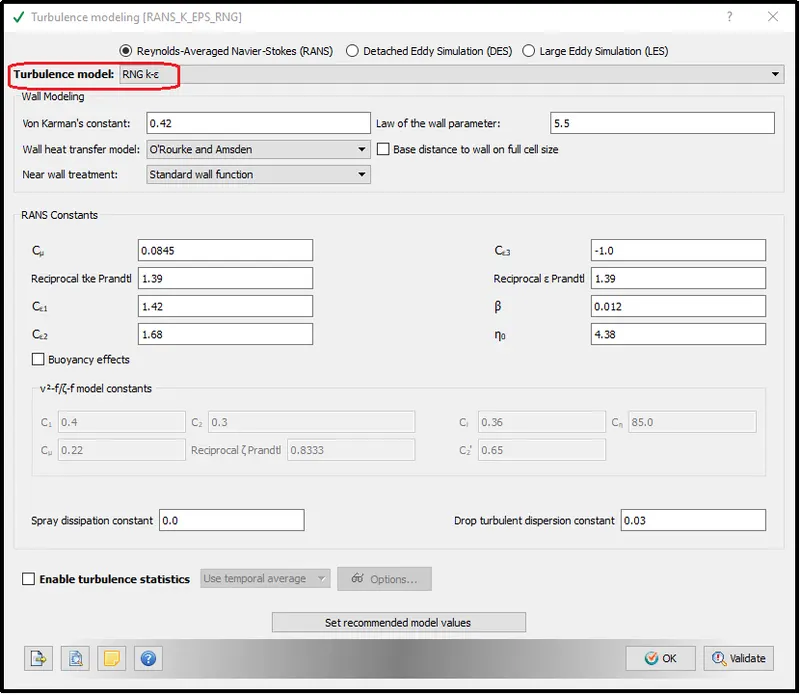
RNG k-epsilon was selected as the turbulence model. which is prefer to get accurate results area further from the walls

Grid control:-

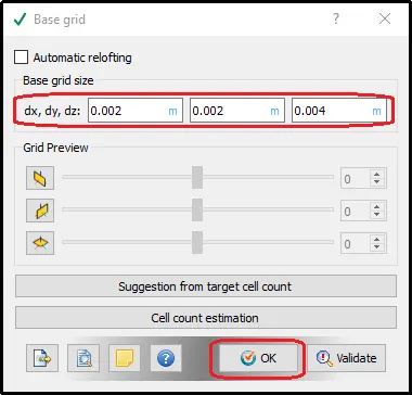
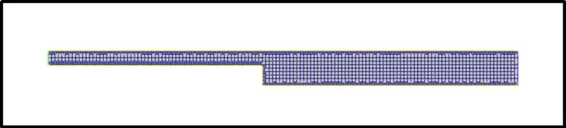
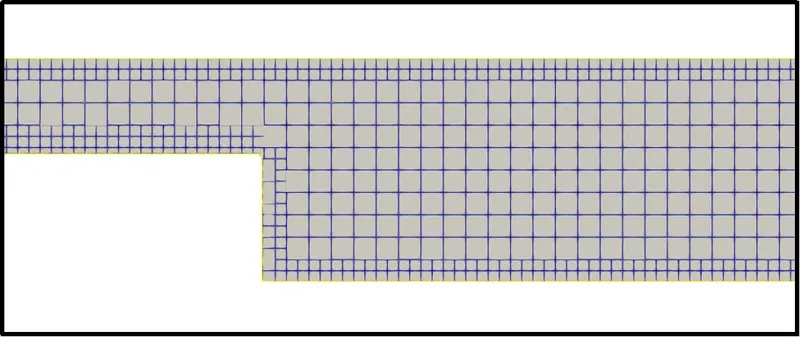
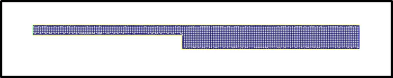
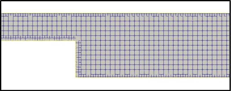
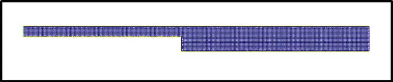
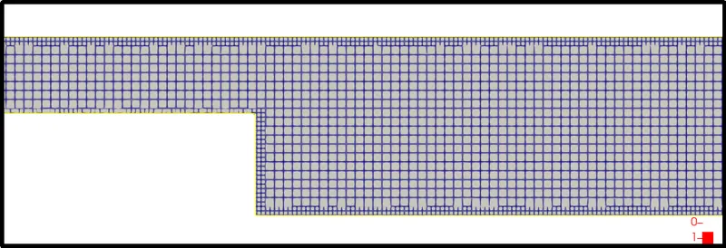
The case setup ran for 3 different grid sizes. As the 2d mesh grid size along Z direction doesn’t matter much in simulation so it was kept as 0.01. It helps us to minimize the number of cell counts without affecting the results.

3 different mesh sizes are:-

For 1^st case

dx = 2e-4m, dy = 2e-4m, dz = 0.01m

For 2^nd case

dx = 1.5e-4m, dy = 1.5e-4m, dz = 0.01m

For 3^rd case

dx = 1e-4m, dy = 1e-4m, dz = 0.01m

Output/Post-processing:-

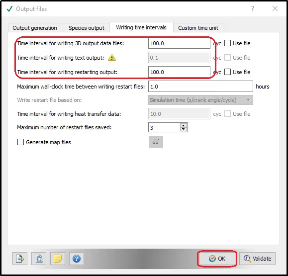
The time interval for writing 3D output data files is kept for 100 cycles i.e. after 100 cycles it will create one 3D output file.

The time interval for writing restarting output was also kept for 100 cycles which will help us restart the simulation in the last count of 100 cycles in case simulation stopped unexpectedly. It helps to save the simulation time of the user.

Export Input files:-

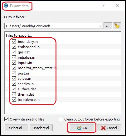
Using file -> Export -> Export Input files all the input files were exported to the simulation folder.

Simulation Run:-

The simulation was run with the help of Cygwin. The directory contains all the export files that were located and using the ‘converge.exe’ setup the simulation was run.

Convergence of Simulaiton:-

Convergence plots for Average Velocity at Outlet:-

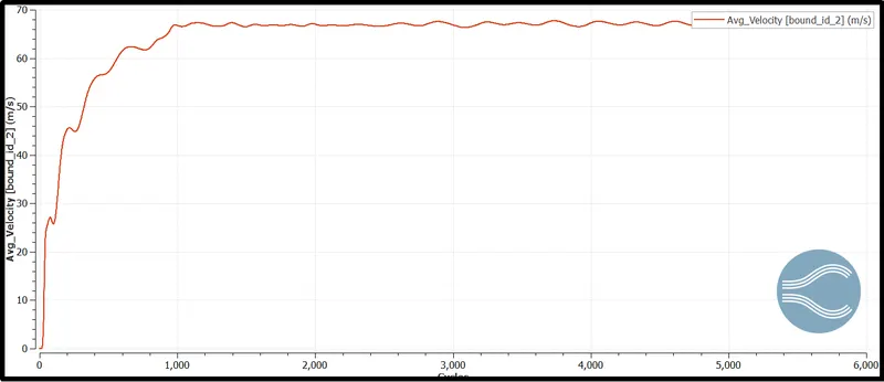
For 1^st case

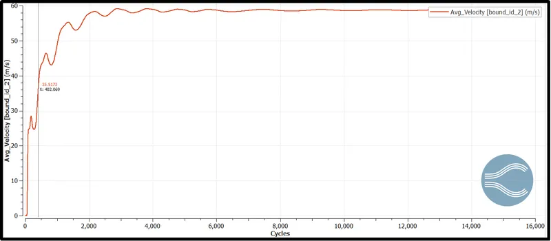
For 2^nd case

For 3^rd case

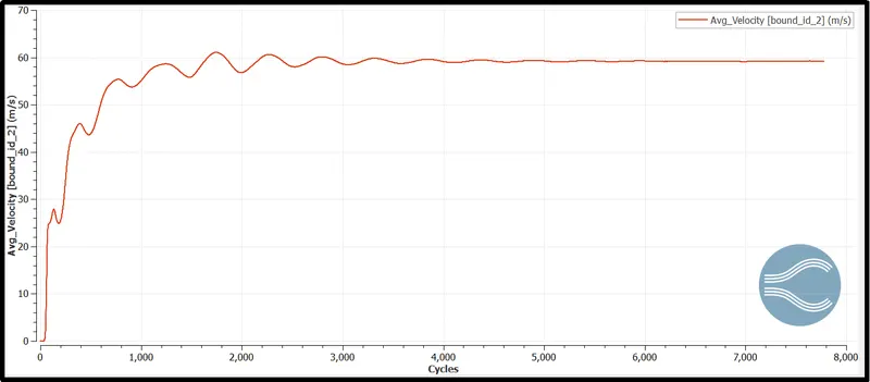
Velocity at the outlet of the backward-facing step model is the important parameter to monitor to get allowable convergence of all results. here we can observe, for all three cases, we are getting proper convergence of the results from our simulation. To get more dependable on our results, it is also important to check the convergence of other parameters such as pressure and mass flow rate of the system.

Convergence plots for Pressure:-

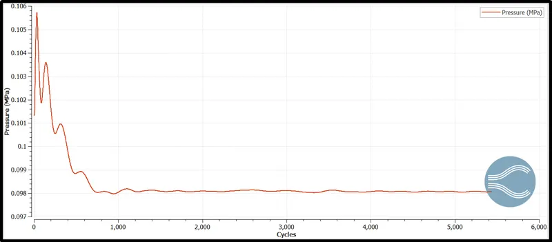
For 1^st case

For 2^nd case

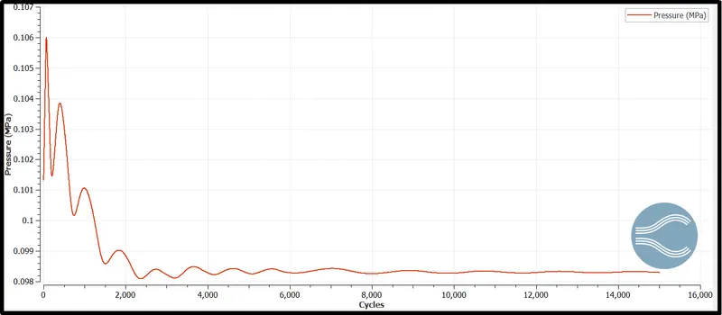
For 3^rd case

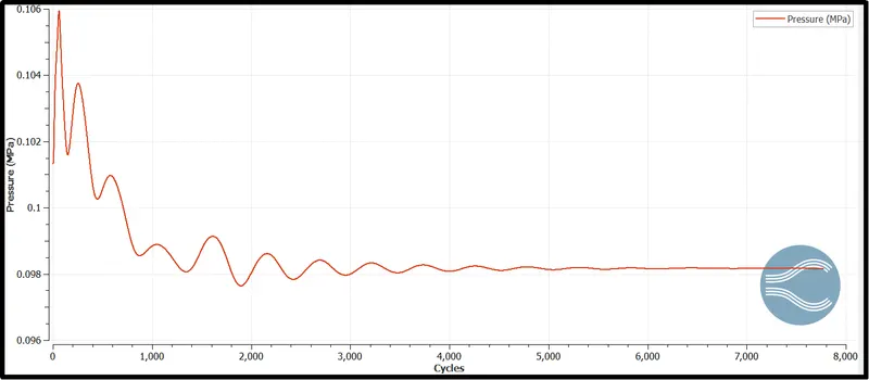
Glimpse over the pressure charts for all three cases of the backward-facing step problem portray almost similar results and also shows the simulation cycles giving the proper converged results for the Pressure values.

Convergence plots for Mass Flow rate at Outlet:-

For 1^st case

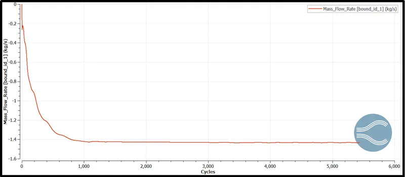
For 2^nd case

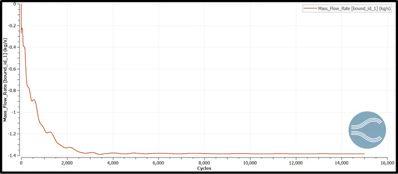
For 3^rd case

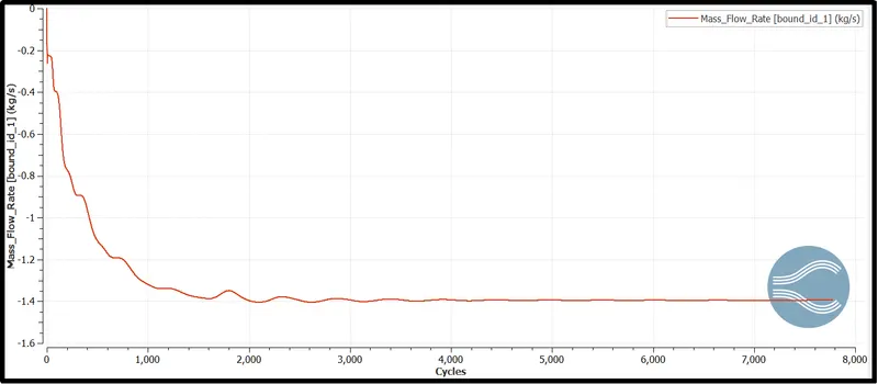
The above figure exhibits the convergence plot of mass Flow rate at the outlet of the backward-facing step model for the above setup. It depicts that for all three cases the results for mass flow rate out are fully converged. For each case, the simulation setup calculating almost the same mass flow out which is always negative.

Total cell count:-

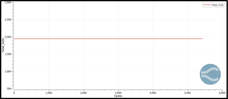
For the first case, the total cell count we are getting using the above setup is 1943.

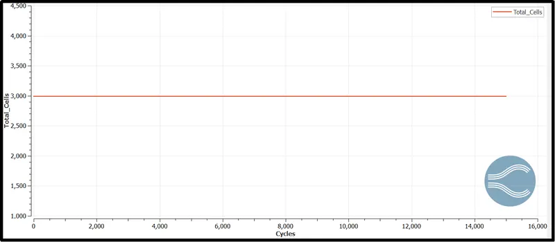
For the second case, it is 3000

And total cell count for the last case is 5516.

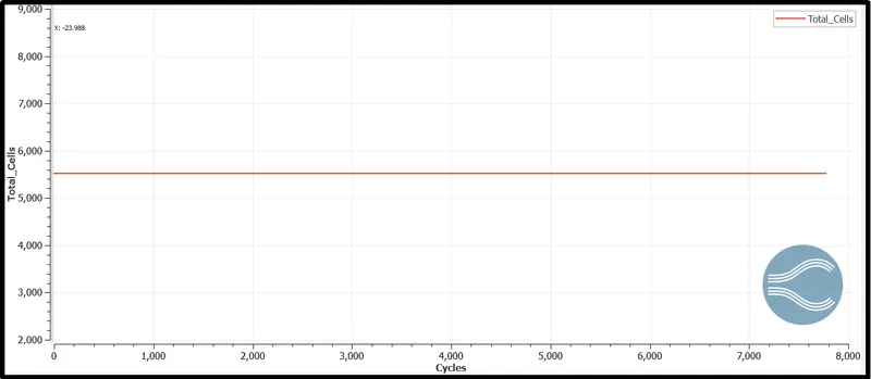
As there is no moving geometry, we used static mesh for the simulation where the cell count remains constant throughout the simulation cycles for all three cases.

Results:-

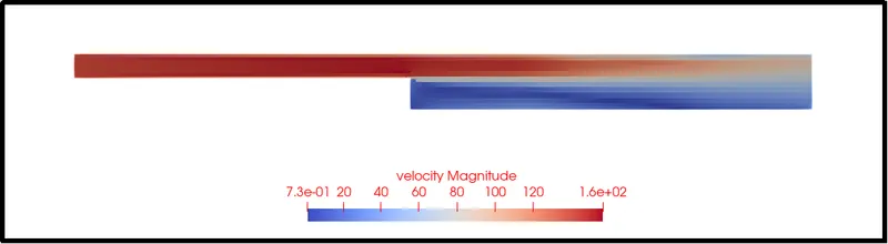
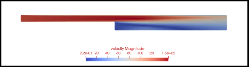
Velocity contour:-

For 1^st case

For 2^nd case

For 3^rd case

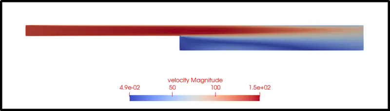
From the observation from each velocity contour, we can find, each simulation providing almost the same velocity plot the only change in result contours is their resolution. the fine grid gives a smooth flow contour than the coarse grid but with a fine grid, computation time increases.

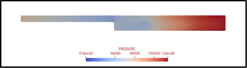
Pressure contour:-

For 1^st case

For 2^nd case

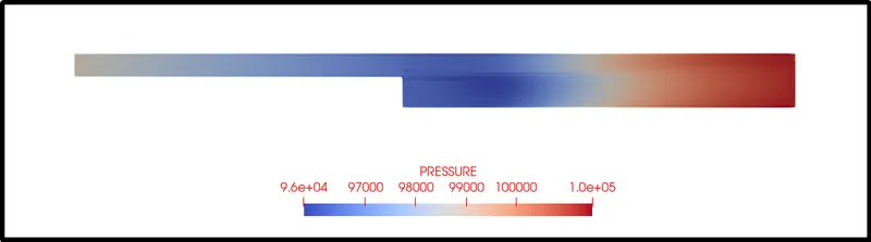
For 3^rd case

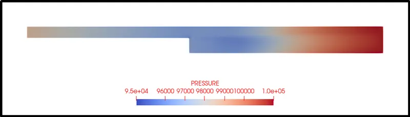
As velocity contour, the pressure contour of all three cases shows the same results except the difference in resolution of the picture.

Velocity Plots:-

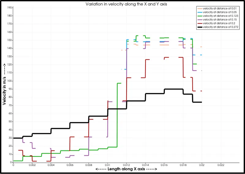
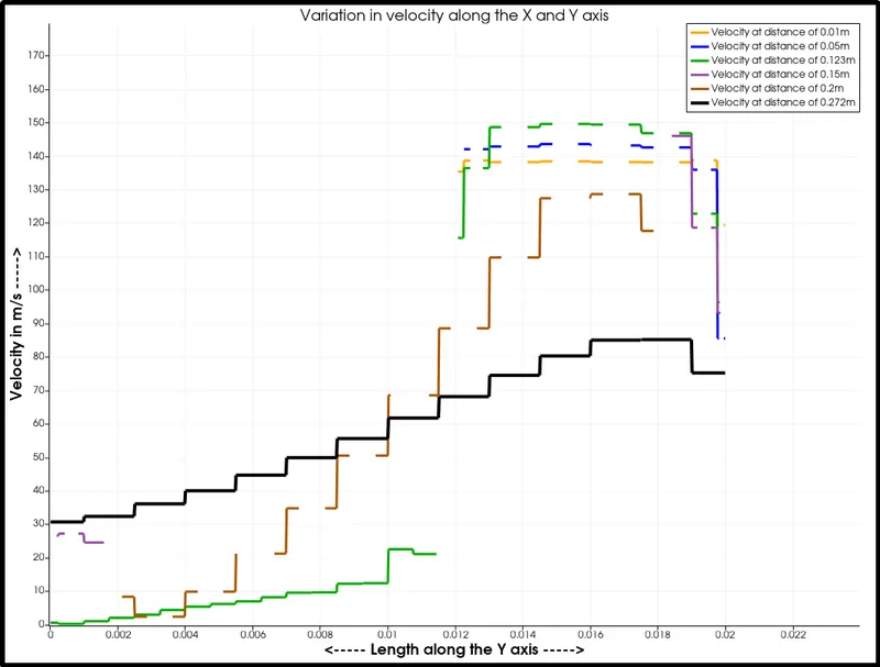
For velocity line graph potted on the line 1,2,3,4,5 and final outlet boundary edge.

For 1^st case

For 2^nd case

For 3^rd case

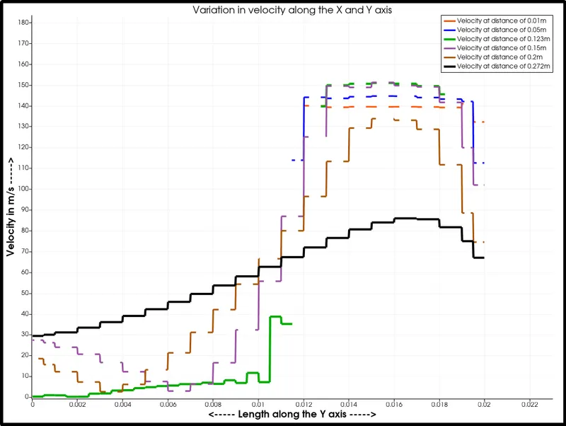
• The above charts portray the line plot for the velocity along the Y-axis and the change in velocity as we move further in the X-direction.
• Glimpse over the graph demonstrates that till the step regio the velocity increasing, which means the reduction in pressure.
• But from the step region, the flow separation happens and, as the area of the flow increases the velocity starts to decreases and pressure starts to increase.

Pressure Plot:-

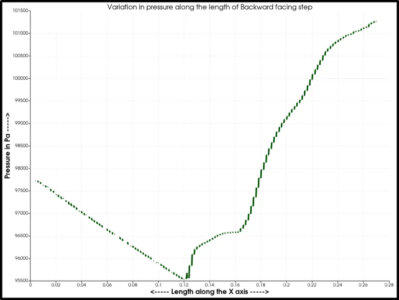
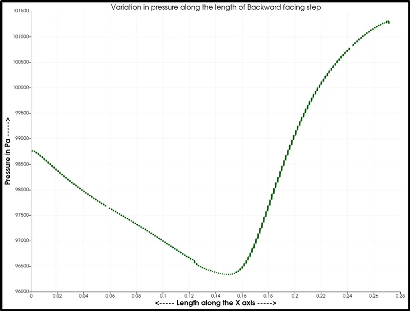
All the Pressure plots were plotted on the horizontal line going toward in X Direction as illustrated in the below figure.

For 1^st case

For 2^nd case

For 3^rd case

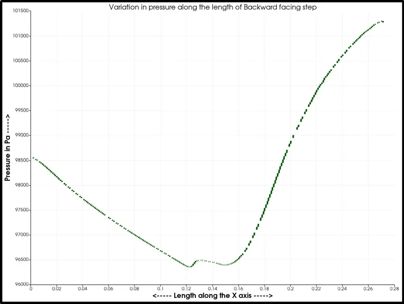
In all the pressure plots, we can observe the slight difference in our results at the step region of the backward-facing step where pressure stops reducing and further starts increasing. From the graph, we can notice, the density of the mesh is a really important factor near the separation of flow. Therefore, with case 3 with fine mesh, we are getting improved results of the variation of pressure.

Flow Separation:-

The separation in the backward-facing step is imposed due to the sharp edge present at the step. In that region the sudden rise in area case the increase in pressure and reduction in velocity and negative pressure near the adjacent side of the step surface.

In this case the high-pressure region on the upper side and negative pressure on the lower side. which leads to the formation of eddies or vortexes adjacent to the surface of the step and flow on the upper side will remain streamline-straight with the reduction in velocity.

we can observe the velocity vector illustrated in the figures, there is turbulent flow in the bottom part and laminar flow in the top part.

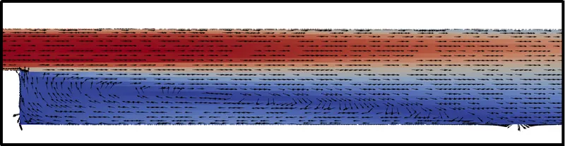
Negative pressure leading to the formation of eddies or vortices near the bottom adjacent area to the step surface and laminar flow near the area to the top surface leads to separation of flow from laminar to turbulent.

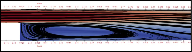
The below figure of streamlined flow exhibits a more detailed representation of the flow separation. as we observe the pressure and velocity plot it shows the sudden changes in flow behavior happening from 0.122m to 0.23m length range.

Observation Table:-

With all the grid sizes we are getting nearly the same results, which means the setup is correct and simulation results are dependable. Thus, results pass the grid independence test.

Conclusion:-

• The backward-facing step (BFS) is considered to be a benchmark geometry for studying detached flow.
• Simulation with low grid resolution simulates the results with minimum time but gives results with little less accuracy and smoothness. Therefore to get an overview of the simulation it is the best choice to run the first simulation with coarse mesh size.
• Simulation with a fine grid preferably uses to perform the final simulation by using the same proven setup.
• simulating the results with different grid sizes is very important to check the mesh independence test.
• Flow separation happens because of the sharp edge of the step and the formation of negative pressure adjacent to the bottom step wall.
• In Flow separation, the flow gets divided into to stream on the top side laminar stream and bottom turbulent steam with eddies formation.
• Separated flows can strongly influence the performance of many industrial devices, such as diffusers, airfoils, air conditioning plants, moving vehicles, and many other industrial systems.

Velocity Animation:-

References:-

[1] Computational simulation of fluid flow over a triangular step using immersed boundary method -https://www.researchgate.net/publication/263794614_Computational_simulation_of_fluid_flow_over_a_triangular_step_using_immersed_boundary_method

[2] Control of the separated flow downstream of a backward-facing step using visual feedback-https://royalsocietypublishing.org/doi/10.1098/rspa.2013.0404