Final Project: Electric Rickshaw modelling
OBJECTIVES:
Create a detailed MATLAB model of an electric rickshaw (three-wheel passenger vehicle) as per the details below:
- Rear wheels driven by PM brushed type motor
- Assume efficiency points of motor controller and motor
- Make an excel sheet of all input and assumed data
- Results: For any three standard driving cycles show energy consumption, the temperature rise of the motor and controller for 100 km constant speed driving at 45 kmph.
INTRODUCTION:
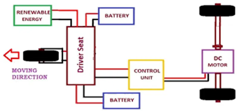
- Electric E-Rickshaw is also known as auto which are going more popular after 2017 in the Indian market. This E-rickshaw is the best alternative to petrol/CNG auto-rickshaw and human or horse-pulled rickshaws because of their low fuel cost, zero emissions and less human efforts.
- The electrical system used in the Indian version is 48VDC can run 90-100 km/full charge, top speed 25 km/hour and this electric motor power ranging from 650-1400 Watts: the battery takes 8-10 hrs to become fully charged. Basic seating capacity is driver plus 4 passengers total of 5 persons.
Components of an EV -
An electric powered car has three primary components - Battery, motor controller, and the electric motor.
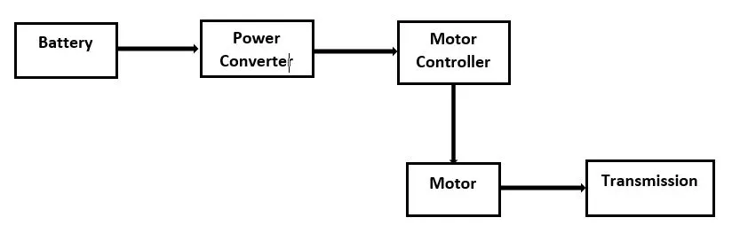
Designing of Electric Motor in Simulink Procedure : While designing we consider the designing in opposite to the flow of power direction .
(1) Vehicle Body Subsystem
- The vehicle is assumed to be a Rear axle driven (3 wheels ).
- The wheels are modelled using simple Tire (Magic formula) simulink blocks.
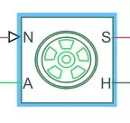
- The N port of the tire corresponds to the Normal Reaction acting on it.
The A port corresponds to the Mechanical Rotational conserving port for the wheel axle. Thus both the wheels on the same axle should form a connection through their respective A ports.
Connection H corresponds to the Mechanical Translational conserving port for the wheel hub through which the thrust developed by the tire is applied to the vehicle. Thus, all the 4 wheels form a connection through their respective H ports and this is in turn connected to the translational hub of the vehicle body.
The connection S represents the output port for slip of the tire.
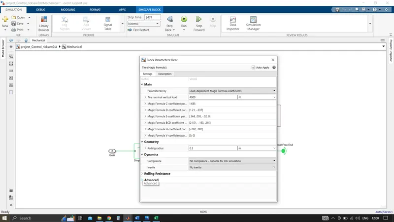
- The tires are parameterized by Peak longitudinal force and corresponding slip.
- The other block parameters such as - rated vertical load, peak longitudinal force at rated load and slip at peak force at rated load - are kept with their default values.
Vehicle Body : This 2 axle (3 wheel) assebly is now connected to a Velocity Body simscape block.
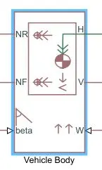
- This block basically represents a two-axle vehicle body in longitudinal motion. The block accounts for -
body mass,
aerodynamic drag,
road incline,
weight distribution between axles due to acceleration
road profile. - Here, the connection H is the mechanical translational conserving port hub.
NF & NR correspond to the output ports for nomral reaction forces on front axle and rear axle wheels respectively.
Connection V represents the actual output translational velocity of the vehicle.
beta is the road inclination angle & W corresponds to the headwind speed (headwind - direction opposite to that of vehicle
- The gross weight is given to be 300 kg.
- The drag force is also considered.
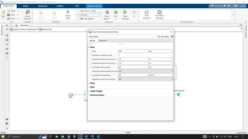
- The pitch dynamics for the vehicle are not considered for this simulation.
The complete Mechanical subsystem is shown below -
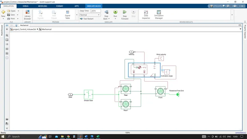
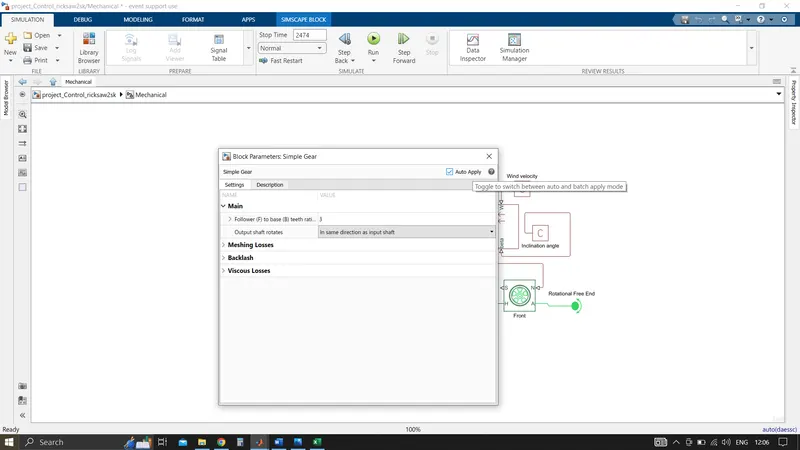
Frontal wheel axel connected to Rotational free end block .
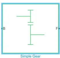
The input for this subsystem is taken as the Rotational speed of the motor. This input is fed to the front axle through a Simple Gear representing the Final Drive Ratio.
Here, the rotational direction of the output shaft is kep the same as that of the input shaft. Also, no meshing losses are considered for the simulation.
) DC Motor :
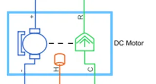
- This block represents the electrical and torque characteristics of a DC motor includes Thermal port to series the temperature of Motor
- The block assumes that no electromagnetic energy is lost, and hence the back emf and torque constants have the same numerical value when in Si units Motor
- Motor parameters can either be specified directly or derived from the no-load speed and stall torque. If no information is available on armature inductance, this parameter can be set to some small non-zero value.
- When a positive current flows from the electrical to-ports, a positive torque acts from the mechanical C to R ports. Motor torque direction can be changed by altering the sign of the back-emf or torque constants.
- The Motor controller will get input from the longitudinal driver. Its tasks are to control the speed of the motor and drive according to the input of the driver.
- Majorly motor controlled we designed had two main parts named PWM voltage generator and H-Bridge Input 1 is getting from the accelmd of a longitudinal driver and it is given to a controlled voltage source block where it is input to the controlled PWM voltage will generate a PWM signal in such a way that H-bridge will generate the required voltage to operate the DC motor for the given driver input
- PWM voltage block negative reference and REF are grounded and REF of H bridge respectively. H-bridge is a motor controller that has IGBT components aligned in the shape of H and will operate only two at a time respectively to the input of the signal from the PWM block.
- When deceleration occurs this H-bridge will give an output from the positive and negative terminals of it. These negative & positive terminals are later connected to the DC motor and battery. All these components are the simscape electrical components so they need a connection to the solver configuration block which helps to solve the simulation.
Parameters
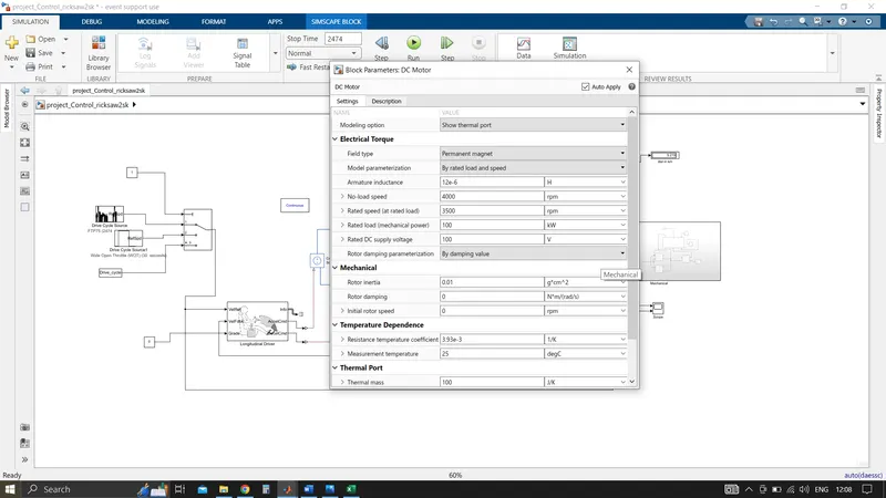
Motor Controller :
- H-Bridge circuit -
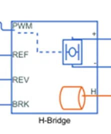
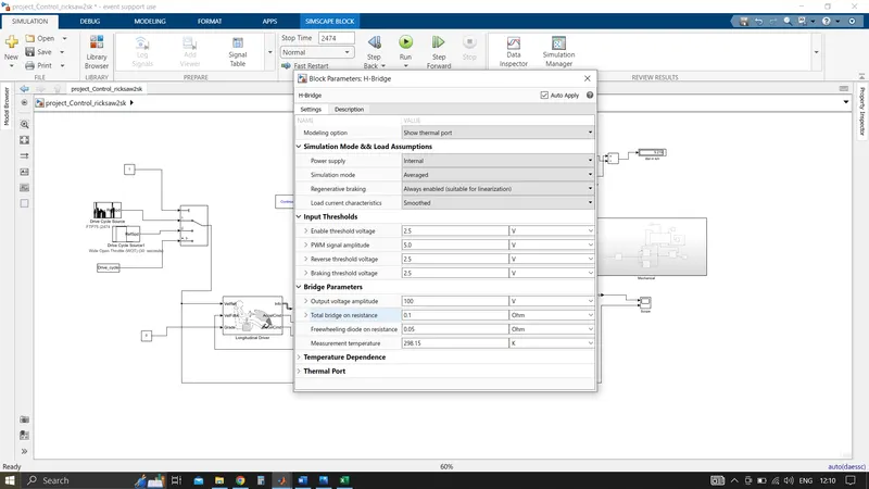
This block represents an H-bridge motor drive. The block can be driven by the Controlled PWM Voltage block in PWM or Averaged mode. In PWM mode, the motor is powered if the PWM port voltage is above the Enable threshold voltage
In Averaged mode. The PWM port voltage divided by the PWM signal amplitude parameter defines the ratio of the on-time to the PWM period. Using this ratio and assumptions about the load, the block applies an average voltage to the load
That achieves the correct average load current. The Simulation mode parameter value must be the same for the Controlled PWM Voltage and H-Bridge block.
- If the REV port voltage is greater than the Reverse threshold voltage, then the output voltage polarity is reversed.
- If the BRK port voltage is greater than the Braking threshold voltage, then the output terminals are short-circuited via one bridge arm in series with the parallel combination of a second bridge arm and a freewheeling diode.
- Voltages at ports PWM, REV and BRK are defined relative to the REF port. If exposing the power supply connections, the block only supports PWM mode.
Parameters:
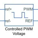
Simulink provides an inbuilt Controlled PWM Voltage block. This block is used for providing the proper pulse inputs to the H-Brdige circuit.
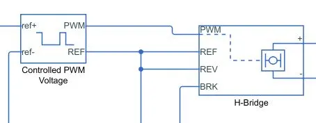
The PWM & REF connections are for the corresponding ports on the H-Bridge circuit.
The 2 reference inputs correspond to the throttle inputs given by the driver. The block generates corresponding pulse width as per the accelerations and brakes apllied by the driver himself.
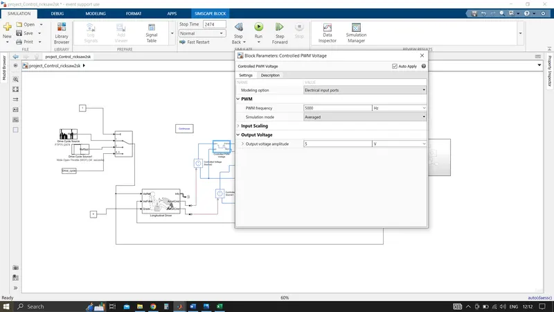
- This block creates a Pulse-Width Modulated (PWM) voltage across the PWM and REF ports. The output voltage is zero when the pulse is low and is equal to the Output voltage amplitude parameter when high.
The duty cycle is set by the input value. Right-click the block and select Simscape Block choices to switch between electrical ref/-ref ports and PS input u to specify the input value.
At time zero, the pulse is initialized as high unless the duty cycle is set to zero or the Pulse delay time is greater than zero.
The Simulation mode can be set to PWM or Averaged. In PWM mode, the output is a PWM signal. In Averaged mode, the output is constant with a value equal to the averaged PWM signal. Select Simulation mode as Averaged.
Parameters
- The H-Bridge circuit along with the PWM input, together form the motor controller circuit.
Temperature Sensor:
- Temperature Sensor is used to measure the temperature of the H-Bridge and Motor.
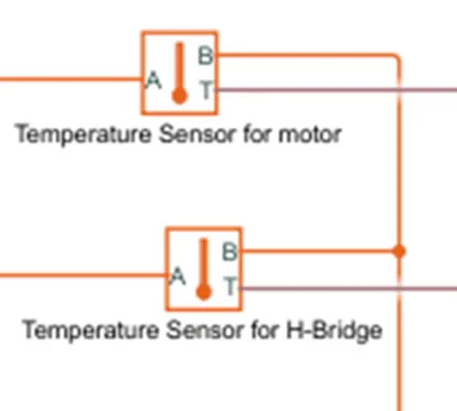
This block measures temperature in a thermal network. There is no heat flow through the sensor. The physical signal port T reports the temperature difference across the sensor.
The measurement is positive when the temperature at port A is greater than the temperature at port B.
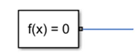
Solver Configuration:
Battery Pack :
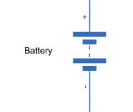
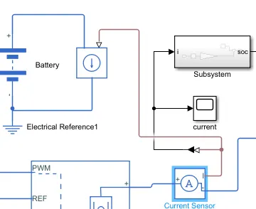
- To model the Battery pack, a simple Battery block is used. This is because, if the generic battery block is used instead, the simulation will run for a much longer time.
- Here, the selected option for Battery Charge Capacity is Finite. Accordingly, the block models the battery as a series internal resistance plus a charge-dependent voltage source.
If the chosen option had been Infinite, the voltage source would have been constant. - Also, the self-discharging of the battery and the battery dynaics are disabled.
- The Battery Nominal Voltage is given as 500V.
The Ampere-hour rating is assumed to be 80.
The rest all paramaters are left with their default values.
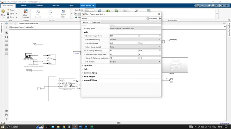
To ensure the battery supplies current as per the requirements of the motor controller and not the rated current, a Current Sensor & Controlled Current Source pair is connected.
(7) Battery State of Charge :
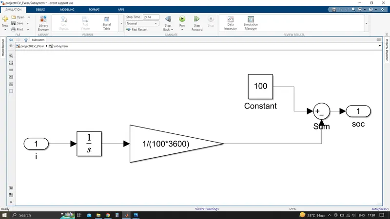
- A small subsystem is created to calculate the State of Charge of the battery.
- This subsystem takes the battery current as the input.
- The essential process to calculate the SOC is by subtracting the charge from the rated capacity of the battery.
- Accordingly, the current is integrated w.r.t. time to get the charge in coulumbs. Now this coulumb value is modified into Ampere hours.
This value is now subtracted from the charging capacity of the battery i.e. 100 Ah. - Finally, the remaining charge is now converted into percentage value of the charging capacity of the battery.
Longitudinal Driver :
- Longitudinal Driver is an inbuilt block provided by the powertrain blockset.
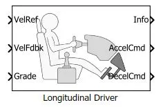
- It is a parametric longitudinal speed tracking controller for generating normalized Acceleration and Braking commands based on reference and feedback velocities.
- The VelRef port is the reference velocity port where the input drive cycle data is fed.
The VelFdbk port corresponds to the feedback velocity. The actual velocity output given by the vehicle body is connected here. By comparing the actual (feedback) velocity with the reference velocity, the driver block generates acceleration and braking signals in order to minimise the error between the two concerned velocities.
Grade corresponds to the grade angle. For this simulation, no inclination is considered and hence, a constant block with value 0 is connected.
Info gives the output for the bus signal for different block calculations like difference in reference vehicle speed and vehicle speed, etc.
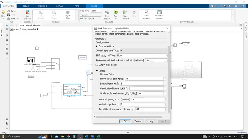
AccelCmd & DecelCmd correspond to the acceleration and deceleration commands generated respectively and are connected to the corresponding ports of the Controlled PWM Voltage block. - Here, the selected control type is PI. Acordingly, the block implements proportional-integral (PI) control with tracking windup and feed-forward gains.
Parameters:
Reference Velocity (Drive Cycle) :
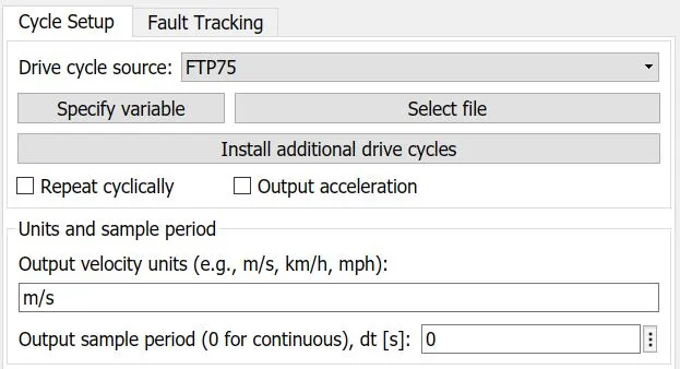
- The Drive Cycle Source block is used to provide the reference speed for the simulation.
- It generates a standard or user-specified longitudinal drive cycle.
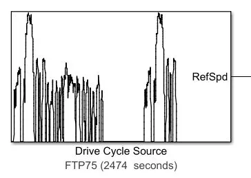
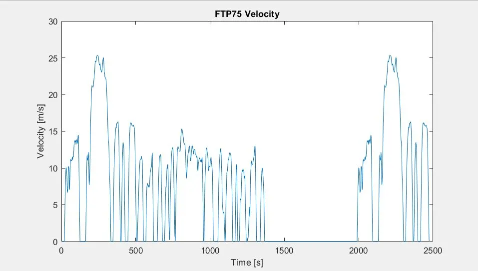
- Here, the selected drive cycle is the standard FTP75.
- The plot of the drive cycle is shown below -
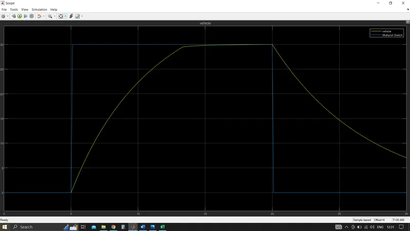
B.Wide Open Throttle (WOT) (60 Seconds):
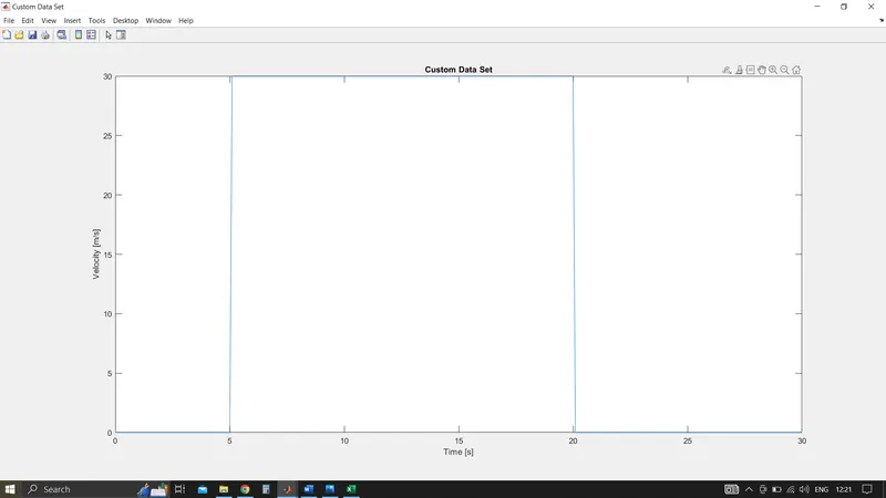
Generates a standard or user-specified longitudinal drive cycle. The block output is the vehicle longitudinal speed. Vehicle speed is 0 for first 5 second, 30m/s for 5 to 20 seconds and zero from 20 to 30 seconds.
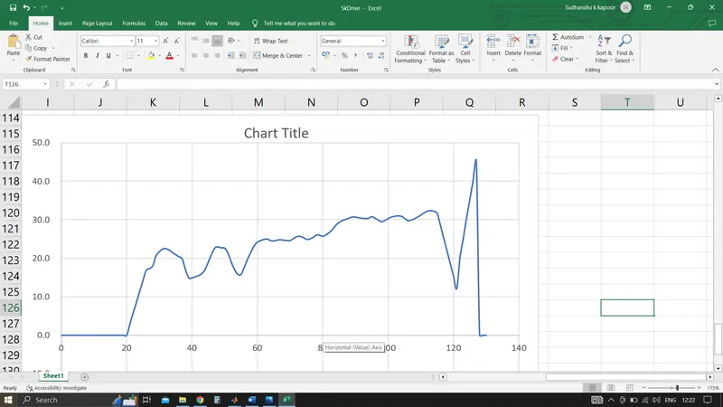
C.User defined cycle:
Results:
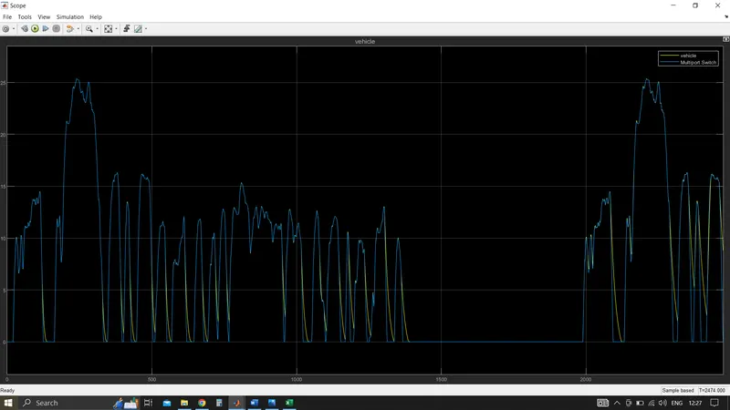
By Running Vehicle with FTP 75 (2474 seconds)
Scope Results for Reference vs Designed vehicle
Temperature :
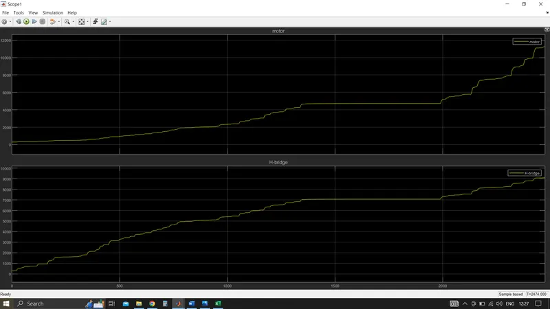
By running the Vehicle with F1P75 Drive cycle for 2474sec the distance travelled is 5.219km
FOR WOT Drive cycle :
Temperature:
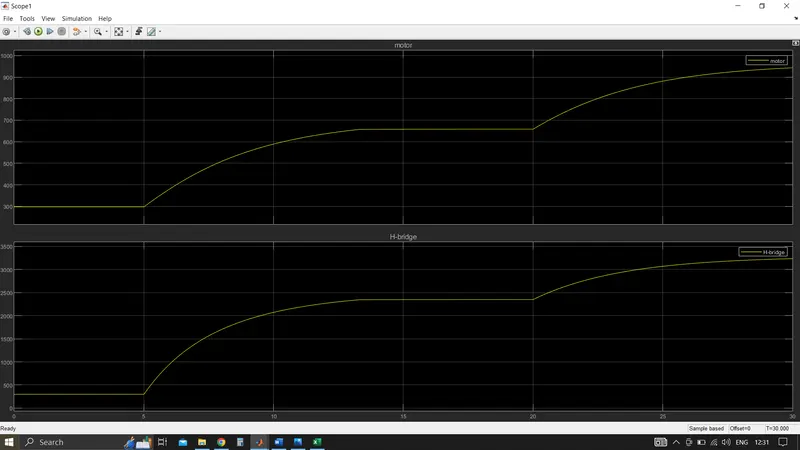
Distance travelled is : 0.1418 km
SOC:
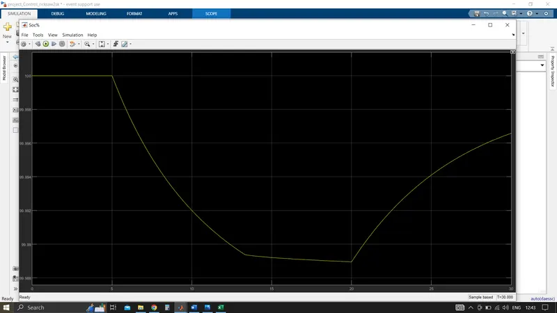
For Manually prepared Drive Cycle:
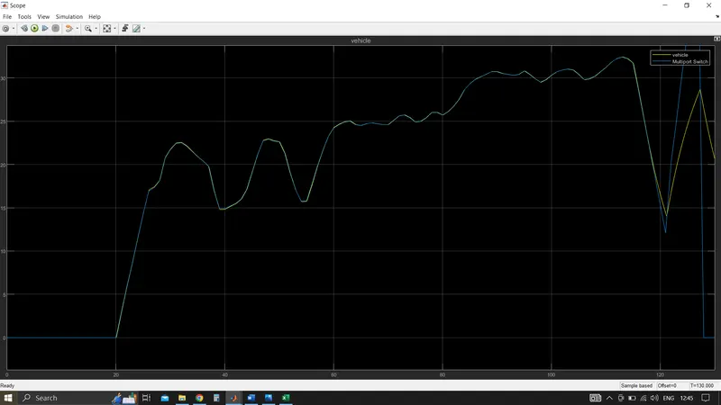
Distance : 0.7249 Km
Temperature:
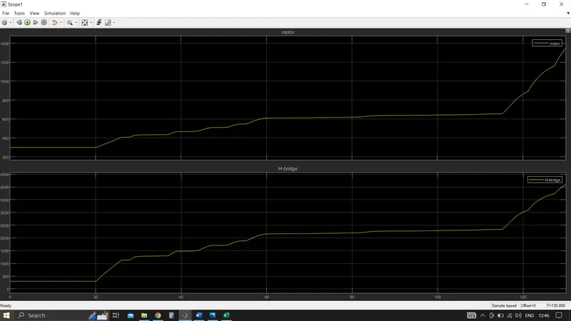
CONCLUSION:
- Here I have compromised with the temperature of Motor and controller to achieve vehicle speed is near to reference speeds. Since I haven't used any cooling system in the model. In the real time application, the motor temperature is less than 100 C
- In the real time application, the motor, battery & controller temperature is controlled by air cooling. Hence, the temperature of this components is not increased to this extent.
- Hence. Created a MATLAB model of an Electric Rickshaw (three wheel passenger vehicle) by using Li-ionbattery, PM Brushed DC Motor.
- Detremined the variations of Temperature of Motor and controller, SoC% and Energy consumed by the by vehicle for all the three Reference Drive cycles (.e: FTP75, WOT, Manually prepared).
- This Battery powered Rickshaw will be the most popular mode of transport in the future.