Final Project: Electric Rickshaw modelling
YOUR ANSWER:
Aim:
To Create a detailed MATLAB model of an electric rickshaw.
Objective:
To Create a detailed MATLAB model of an electric rickshaw for the following condition:
1.Rear wheels driven by PM brushed type motor.
2.Assume efficiency points of motor controller and motor.
3.For any three standard driving cycles show energy consumption, temperature rise of motor and controller for 100 km constant speed driving at 45 kmph.
Introduction:
In India, Rikshaw is mainly used for public transport. A typical rikshaw is three-wheeler vehicle with driver+3 passenger arrangement. In this project, we are designing a Rear wheel driven electric rickshaw using permanent magnet brushed type motor with payload of 300 kg.
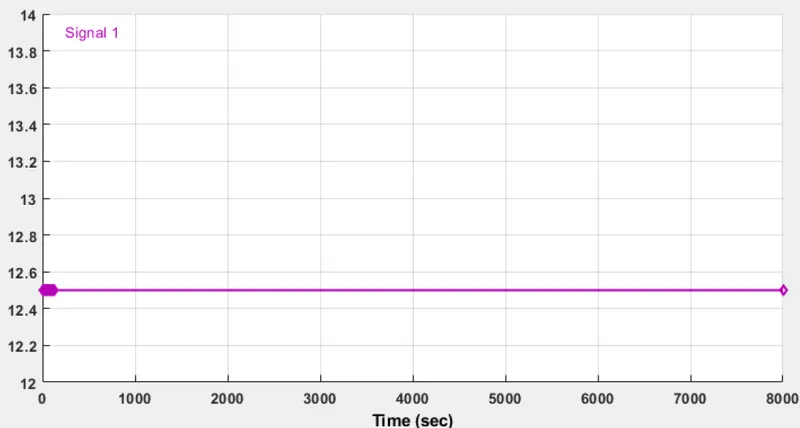
Important result to be obtained is the rise in temperature of motor and controller when the vehicle has travelled 100km distance at 45kmph constant speed throughout. For this a separate drive cycle is created. In this drive cycle the speed is 12.5m/s constant for 8000 seconds. With speed of 12.5m/s for 8000 seconds, the vehicle should complete 100km.
Procedure:
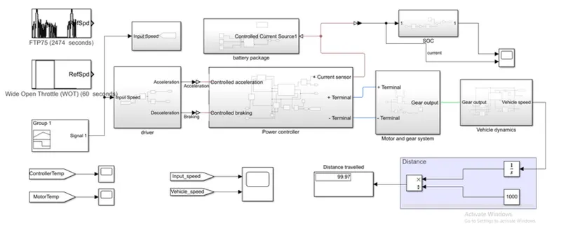
An electric autorickshaw should have the following components to simulate in virtual environment:
1.Drive cycle
2.Battery
3.Driver Configuration
4.Power Controller
5.Motor and Gear system
6.Vehicle Dynamics
An electric rikshaw is combination of above-mentioned subsystems.
Block diagram of electric rikshaw is as follows:
Drive cycle:
A driving cycle is a series of data points representing the speed of a vehicle versus time. they are used in propulsion system simulations to predict performance of internal combustion engines, transmissions, electric drive systems, batteries, fuel cell systems, and similar components. Here we are using two standard drive cycle:
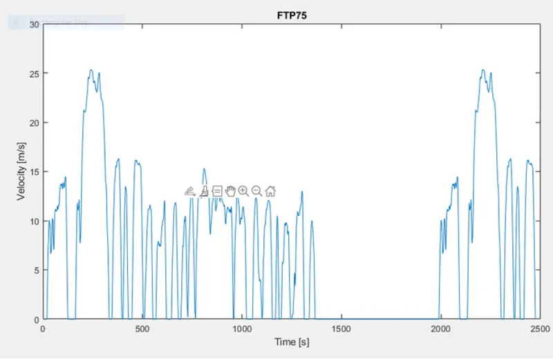
A.FTP75 (2474 cycle):
The Federal Test Procedure (FTP) is composed of the UDDS followed by the first 505 seconds of the UDDS. Though it was originally created as a reference point for fossil fuelled vehicles, the UDDS and thus the FTP-75, are also used to estimate the range in distance travelled by an electric vehicle in a single charge.
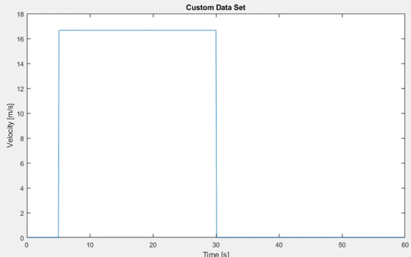
B.Wide Open Throttle (WOT) (60 Seconds):
Generates a standard or user-specified longitudinal drive cycle. The block output is the vehicle longitudinal speed. Vehicle speed is 0 for first 5 second, 60kmph for 5 to 30 seconds and zero from 30 to 60 seconds.
C.User defined cycle:
This cycle has a constant speed of 45kmph or 12.5m/s for 8000 seconds. The reason of the time being 8000 seconds is that the vehicle will take 8000 seconds for completing 100km ride at 45kmph speed.
Battery Package:
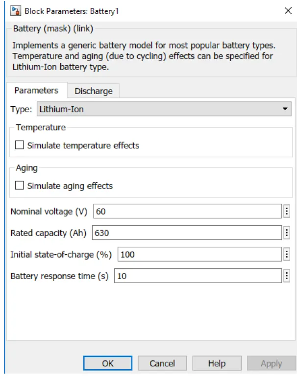
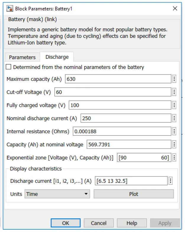
The battery used is a lithium-ion battery of 60V and 630Ah capacity. The output of the battery is its current, SOC, and voltage. A controlled current source drives the battery to charge and discharge. The input for this controlled current source is the current from the Power controller block.
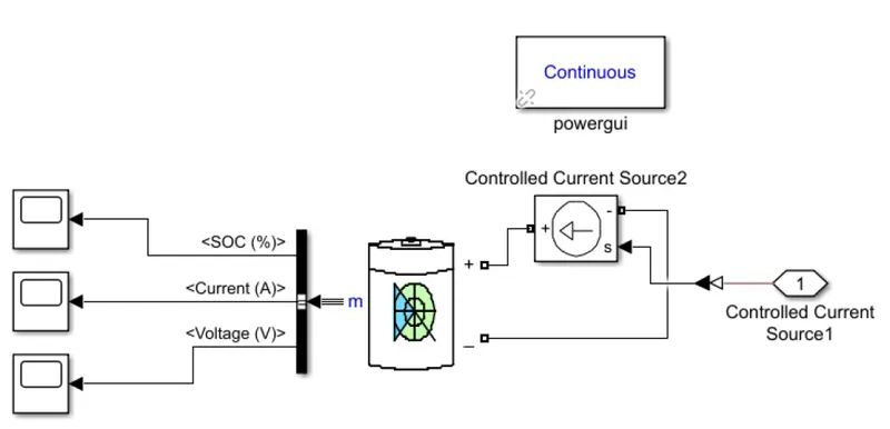
The temperature effects are not simulated for battery.
Driver:
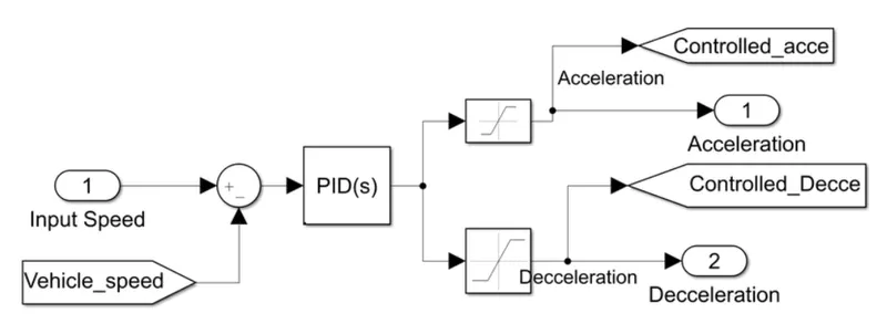
This subsystem compares the input speed and the vehicle speed. If the output is positive speed accelerating command is given from the controller. If the output is negative, deceleration command is given from the controller output. This output is controlled by saturation blocks by giving the upper and lower limits.
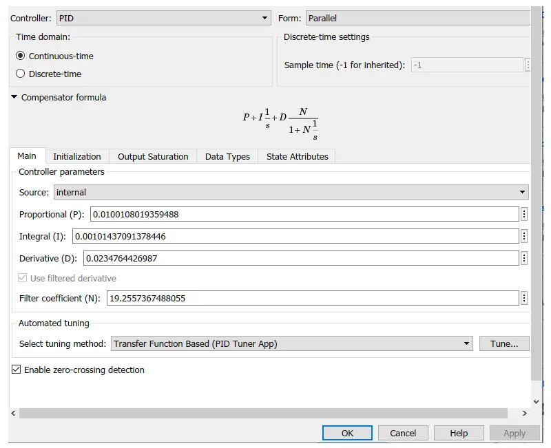
The PID controller is tuned and is a continuous time based.
Power Controller:
Power controller block has prime significance in the electric powertrains. It consists of controlled PWM voltage block, H-bridge block, two controlled voltage source, current sensor and temperature sensor.
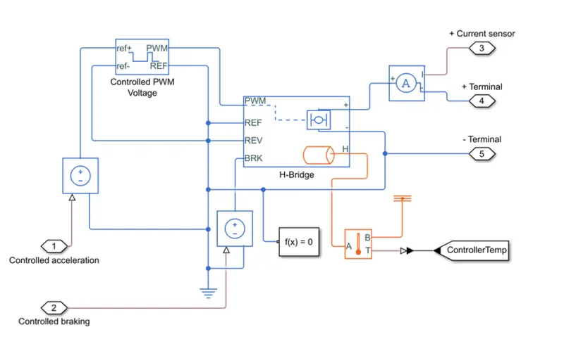
Controlled acceleration from driver subsystem is provided to controlled voltage source, the controlled voltage source converts the input of controlled acceleration signal to the equivalent voltage signal and output of controlled voltage source is provided to controlled PWM voltage block. Similarly, controlled braking signal is provided to another controlled voltage source and output of controlled voltage source is provided to H-bridge block.
Controlled PWM Voltage:
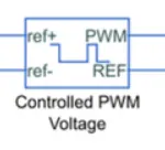
The Controlled PWM Voltage block represents a pulse-width modulated (PWM) voltage source. The block calculates the duty cycle based on the reference voltage across its ref+ and ref- ports.
H-bridge:
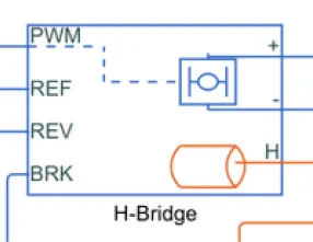
This block represents an H-bridge motor drive. The block can be driven by the Controlled PWM Voltage block in PWM or Averaged mode. In PWM mode, the motor is powered if the PWM portvoltage is above the Enable threshold voltage. In Averaged mode, the PWM port voltage divided by the PWM signal amplitude parameter defines the ratio of the on-time to the PWM period.Using this ratio and assumptions about the load, the block applies an average voltage to the load that achieves the correct average load current. The signal at the REV port determines the polarity of the output. If the value of the signal at the REV port is less than the value of the Reverse Threshold Voltage parameter, the output has positive polarity; otherwise, it has negative polarity.
Thermal Sensor:
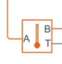
The Temperature Sensor, a device that determines the temperature differential measured between two points without drawing any heat. Connections A and B are thermal conserving ports that connect to the two points where temperature is being monitored. Port T is a physical signal port that outputs the temperature differential value. Output from H port from H-bridge block is given to port A.
The measured temperature is determined as T = TA – TB.
Motor and Gear system:
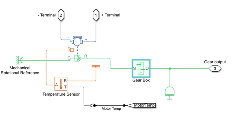
+ and – terminal output from power controller block is connected to respective terminals of DC motor
DC motor:
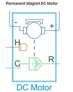
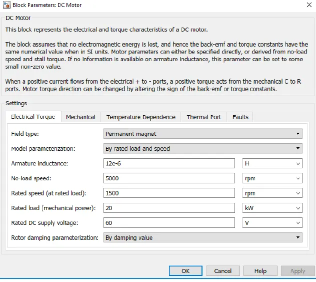
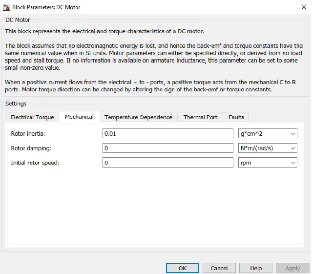
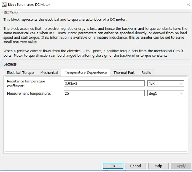
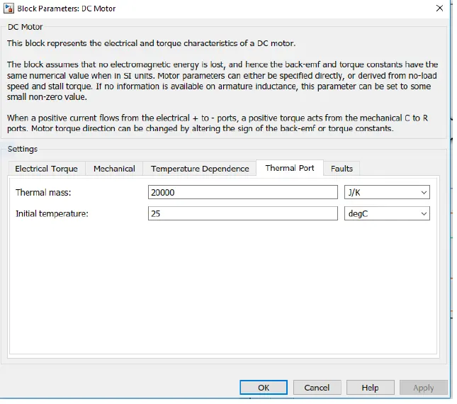
The block assumes that no electromagnetic energy is lost, and hence the back-emf and torque constants have the same numerical value Motor parameters can either be specified directly, or derived from no-load speed and stall torque. H port output from DC motor is provided to temperature sensor and shown on scope as motor Temp. Mechanical rotational reference block is used to connect mechanical rotational ports that are rigidly affixed to ground.
Gear Box:
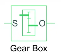
The gear box is characterized by its Gear ratio. The gear ratio is determined as the ratio of the input shaft angular velocity to that of the output shaft. Here Gear ratio is 5.
Vehicle Dynamics:
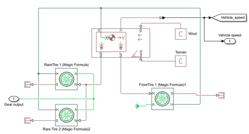
Vehicle dynamics subsystem is simply the vehicle body working to the given task. It has wheels road conditions, surrounding conditions, load on the vehicle etc.
Vehicle body:
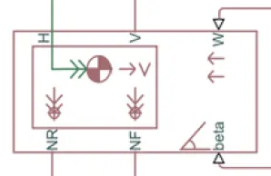
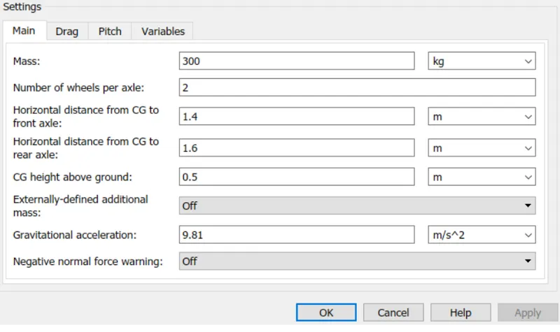
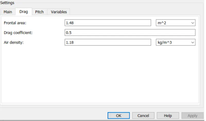
Represents a two-axle vehicle body in longitudinal motion. The block accounts for body mass, aerodynamic drag, road incline, and weight distribution between axles due to acceleration and road profile. Optionally include pitch and suspension dynamics or additional variable mass and inertia. The vehicle does not move vertically relative to the ground.
Connection H is the mechanical translational conserving port associated with the horizontal motion of the vehicle body. The resulting traction motion developed by tires should be connected to this port. Connections V, NF, and NR are physical signal output ports for vehicle velocity and front and rear normal wheel forces, respectively. Wheel forces are considered positive if acting downwards. Connections W and beta are physical signal input ports corresponding to headwind speed and road inclination angle, respectively. If variable mass is modelled, the physical signal input ports CG and M are exposed. CG accepts a two- element vector representing the x and y distance offsets from vehicle CG to additional load mass CG. M represents the additional mass. If both variable mass and pitch dynamics are included, the physical signal port J accepts the inertia of the additional mass about its own CG.
Tyres:
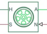
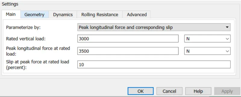
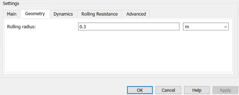
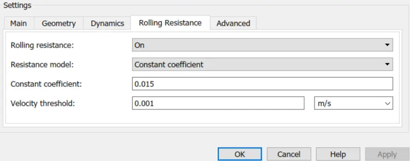
Tyre block Represents the longitudinal behaviour of a highway tire characterized by the tire Magic Formula. Connection A is the mechanical rotational conserving port for the wheel axle. Connection H is the mechanical translational conserving port for the wheel hub through which the thrust developed by the tire is applied to the vehicle. Connection N is a physical signal input port that applies the normal force acting on the tire. The force is considered positive if it acts downwards. Connection S is a physical signal output port that reports the tire slip. Optionally expose physical signal port M by right-clicking on the block and selecting Simscape block choices to switch between variants. Physical signal port M accepts a four-element vector corresponding to the B, C, D, and E Magic Formula coefficients.
Result:
1.FTP75:
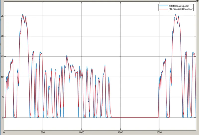
Input speed vs output speed:
The modelled rickshaw efficiently follows the input drive cycle.
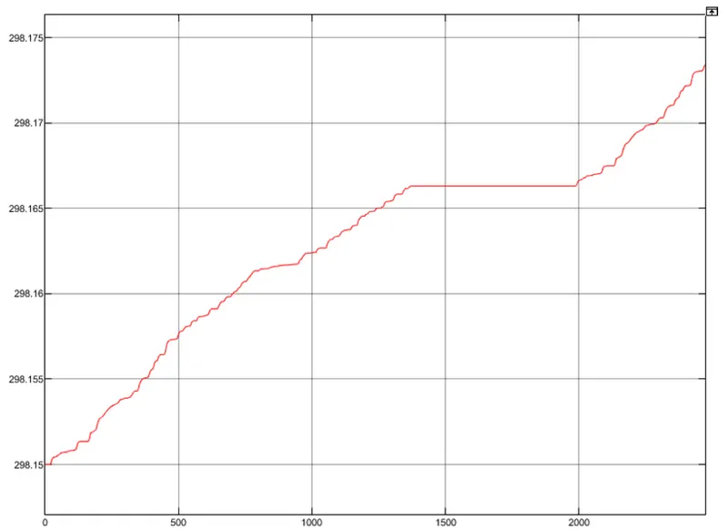
Controller temperature:
Temperature of controller rises when the vehicle is running and is constant when it stops. Rise in Temperature is negligible.
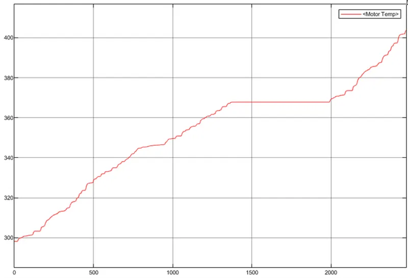
Motor temperature:
Motor temperature is increased by 100 deg. K when in operation.This rise of temperature is very high and need to be controlled. It can be concluded that cooling medium is necessary for this powertrain for efficient working and durability.
SOC and Current:
SOC is reduced to 79%, which was 100% at start of the drive. SoC plot is constant whenever vehicle is stops and rise in the curve is seen due to regenerative braking.
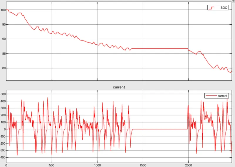
AS per the drive current follows positive and negative profile. Positive being current drawn from the battery and negative being current drawn inside the battery(regeneration). That is where the SOC increases. Also, it is zero for zero speed between 1400 and 2000 seconds (approx.) span.
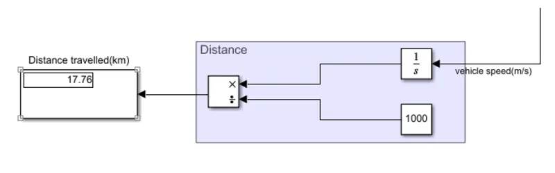
Distance travelled: 17.76 km
2.WOT (wide open throttle) (60kmph reference speed for 30 seconds):
Input speed vs output speed:
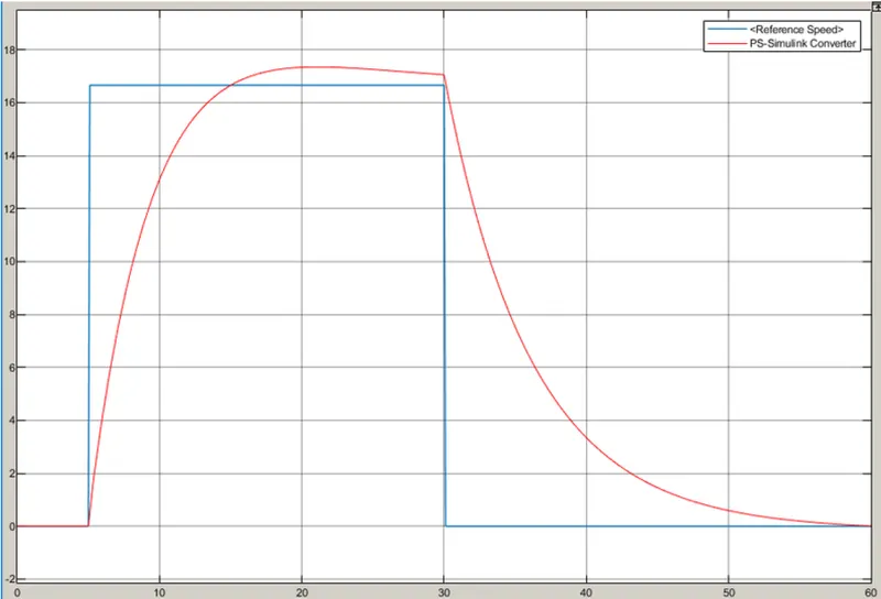
The output speed tried to follow the input and before reaching the specified speed throttle was released from full to zero. The rickshaw could not reach reference speed of 60kmph within 30 seconds. Also, to reach zero after wot is released, it took next 30seconds to reach zero (to stop).
Controller temperature:
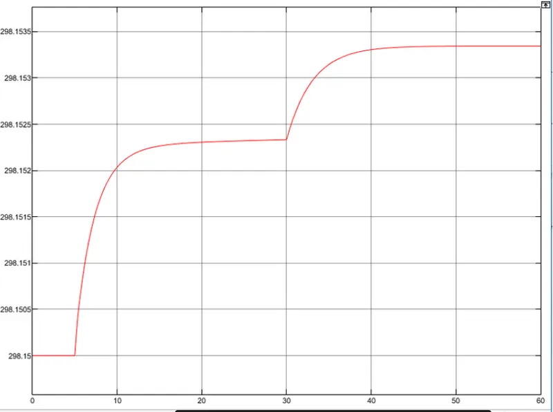
Temperature of controller is constant for first 5 seconds as there is no input and vehicle is at rest. As the vehicle starts to follow the wot condition, the temperature drastically increases. When it reaches above 60kmph and now tries to settle, temperature is also settled to some extent and no rise is seen in it. Again, during deceleration same behaviour is seen. Rise in Temperature is negligible.
Motor temperature:
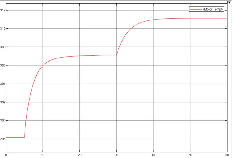
It has reached to 311 kelvin which was 298 kelvin at start.
SOC and Current:
At constant zero speed, SOC is 100% for first 5 seconds.As vehicle starts running for 30 seconds ,SOC drops to 98.25 and then again rises back to 99.5 in next 30 second ass brakes are applied.
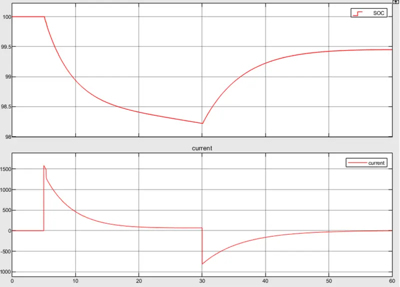
For current, it is zero for zero speed (at rest), positive (drawn from battery) till 30 seconds and it is negative (drawn to battery) for 30 to 60 second period.
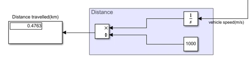
Distance travelled: 0.47km
3.User Defined cycle (45kmph for 100km):
Input speed vs output speed:
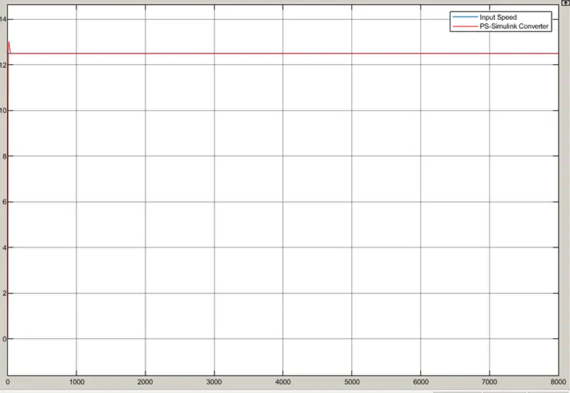
Above plot describes the control accuracy of the system. Input speed and output speed is very identical, meaning the controller is performing its function accurately. Constant speed of 45 kmph (12.5m/s) is achieved throughout the 100km distance
Controller temperature:
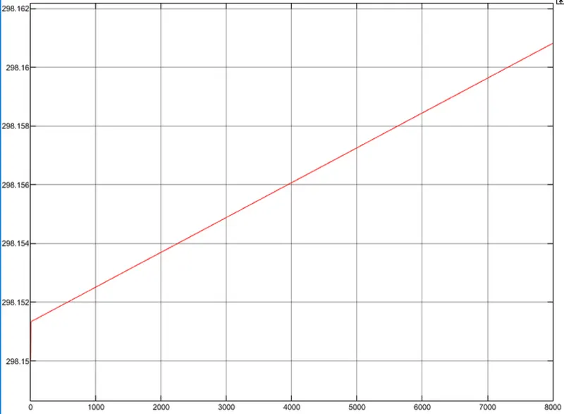
During the 100km travel of the vehicle at constant 45 kmph speed, the controller temperature has risen from 298.15 to 298.161 kelvin. There is negligible rise in the controller temperature.
Motor temperature:
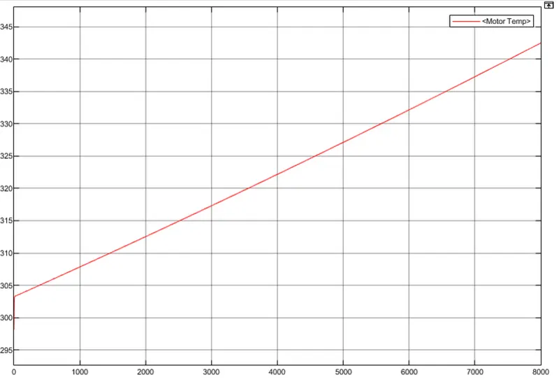
For 0 to 45kmph acceleration, temperature rise was 298 to 304 kelvin. As vehicle complete 100 km distance the motor temperature reached 343 kelvin.
SOC and Current:
The SOC of the rickshaw which was 100% at start, reached to 0% at the end of 100km.
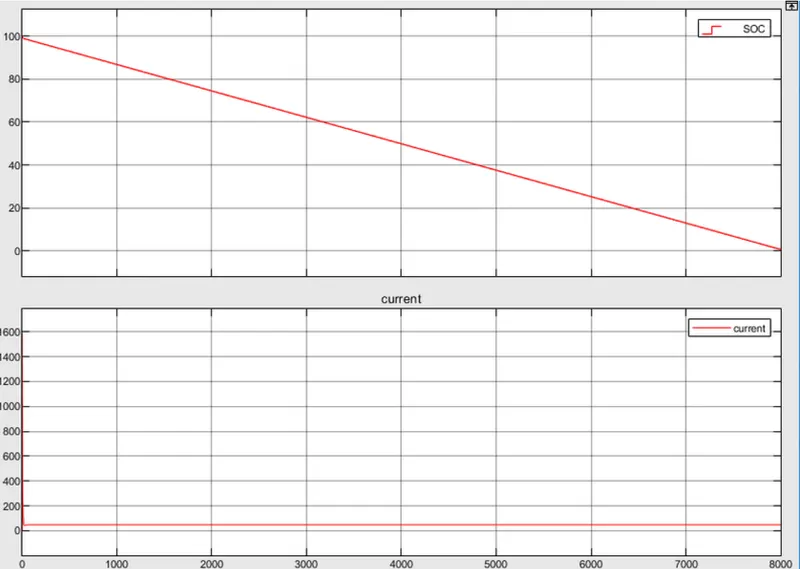
The current drawn from the battery is also constant throughout. Also, the current is only in positive direction. This is because the speed never changes and there is not deceleration. If there was any deceleration, there would be current regeneration and battery would be charged resulting in negative current.
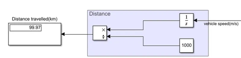
Distance travelled:100km
Conclusion:
MATLAB model of an electric Rickshaw is created. It is simulated for three driving cycles and its results are analysed.