Final Project: Electric Rickshaw modelling

AIM : Create a detailed MATLAB model of an electric rickshaw (three wheel passenger vehicle) and Make an excel sheet of all input and assumed data

GIVEN: Rear wheels driven by PM brushed type motor

Assume efficiency points of motor controller and motor

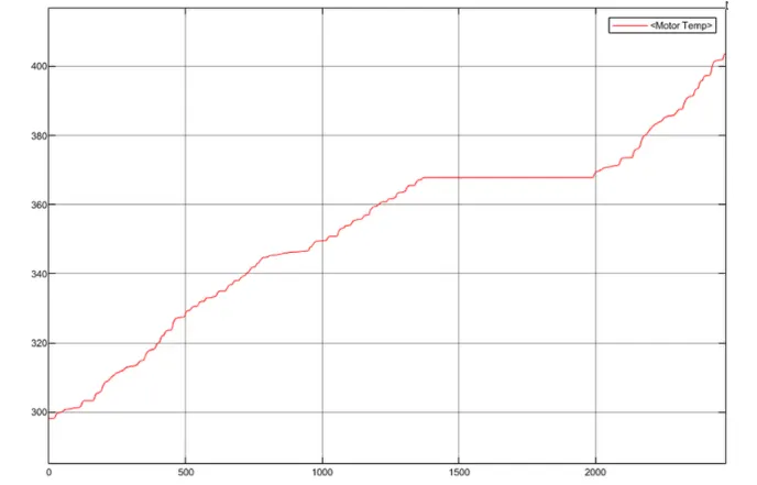
For any three standard driving cycles show energy consumption, temperature rise of motor and controller for 100 km constant speed driving at 45 kmph.

ANSWER:

E-rickshaw development started in the global market sometime during World War period, but faded away with time. These were later introduced in China by local and Japanese motor vehicle industries further spreading in areas of Asia.ln India development of e-rickshaw started in late 1990s with the aim of improving manual rickshaws. E-rickshaw was developed with motor assisted pedal rickshaw (MAPRA) by Nimbkar Agricultural Research Institute (NARI). ELECSHA (electric rickshaw) 2000 was also developed later on, but there were issues with battery performance and quality, due to which these could not trend in market

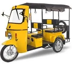
Electric E-Rickshaw is also known as electric tuk-tuft e-rickshaw and auto which are going more popular after 2018 in Indian market. This E-rickshaw is best alternative of petrol/ CNG auto rickshaw and human or horse pulled rickshaws because of their low fuel cost, zero emissions and less human efforts. The electrical system used in Indian version is 48VDC can run 90- 100 km/full charge, top speed 25 km/hour and this electric motor power ranging from 650-1400 Watts; the battery takes 8-10 hrs to become fully charged. Basic seating capacity is driver plus 4 passenger total 5 persons. Here basically, e-rickshaw is designed in CREO and MATLAB Simulink. In the designed electric rickshaw main blocks are battery, drive cycle, controlled, DC Motor, Vehicle body and transmission system. Drive cycle is the input of human effort that how he is going to drive his actual cycle. We can use drive cycle like FTP75, WOT or by using Excel. The main objective of this project is to obtain speed by driver, to estimate the temperature of motor and controller, to estimate the state of charge (SOC) and distance travel by the vehicle. There is a SOC block that will estimate the state of charge of battery, distance is calculated by speed and time parameter for all the three Drive cycle

.

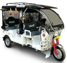
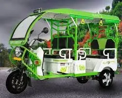
In 1999, Mahindra launched its first electric 3-wheeler.19 Around 2010, E-rickshaws gained prominence in various urban and semi urban areas of UP, Bihar, West Bengal and cities of some other states. Delhi NCR also witnessed a rise in number of e-rickshaws during Commonwealth Games20. E-rickshaws were launched in Delhi with the objective to eventually phase out conventional cycle rickshaws; this objective was eventually altered when e-rickshaws were excluded from NMT category and included in Motor Vehicles Act (2014) as last mile connectivity modal option.
As per Motor Vehicles Act 2014 and Motor Vehicles (amendment), e-rickshaws are defined as A special purpose battery operated vehicle having three wheels and intended to provide last mile connectivity for transport of passengers for hire or reward, provided, such vehicle is constructed or adapted to carry not more than four passengers, excluding the driver, and not more than 40kg luggage in total; net power of its motor is not more than 4000 W and maximum speed of the vehicle is not more than twenty-five kilometer per hour.

E-Rickshaws are the latest entry in the Indian road and transport system. A flexible, non-polluting and affordable system, they have been playing a significant role in solving the last mile connectivity issue. Due to the absence of rules and norms, they have been largely operating very informally. White the licensing of E-Rickshaws has been given the nod by the Ministry of Road Transport and Highways, the operation of this system is still ambiguous which has currently led to the ban order by the Delhi High Court There exists the issue of monitoring and framing the rule book for E-Rickshaws for the safety and security of the commuters using these systems. Policy guidelines are required on whether E-Rickshaws are an Intermediate ParaTransit (IPT) system, who is responsible for the licensing and regulation and how it gets integrated and act as feeder to the public transport. Specific provisions are required to address questions on speed, vehicle specifications,insurance, lane traffic and fare charges. This requires a policy framework to address the concerns of both erickshaw drivers and its counterparts.
Centre for Public Policy Research (CPPR) believes that ERickshaw needs to be integrated into the system at the policy as well as at the infrastructure level and developed as an appropriate feeder system. This demands for a need based assessment and defining of IPT Characteristics in the current public transport system of India. This policy brief aims to develop an approach wherein which systems like erickshaw shall be formally integrated and devised to support the existing systems and enable a sustained transport system.

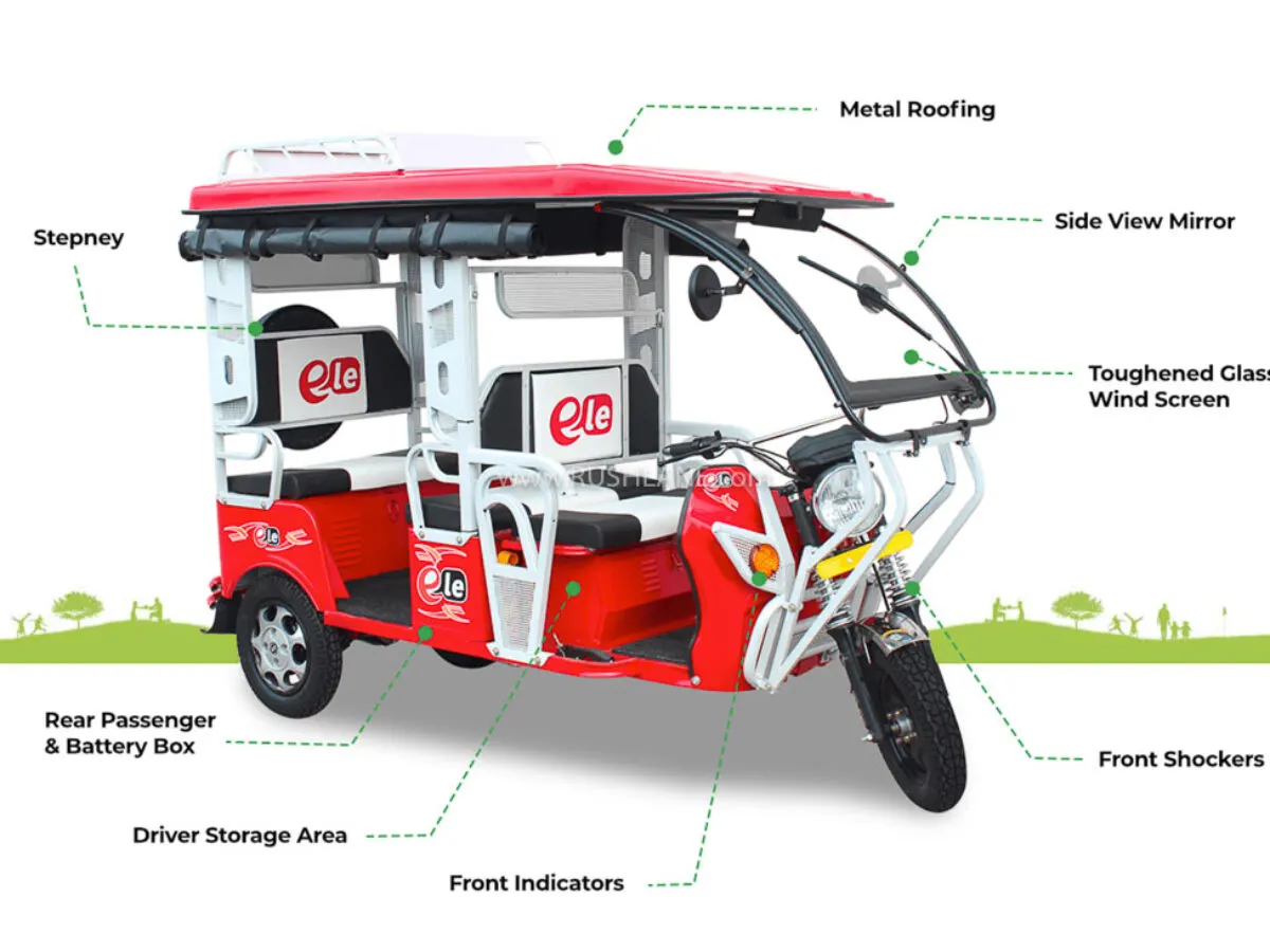
General detail of E-Rickshaw
• Battery Type Lithium Ion 60.8 V 160 Ah

• Vehicle kerb weight 260 kgs

• Load capacity 340 kgs

• Vehicle speed 45 kmph

• Driving range 100 km (160 Ah)

• No of wheels per axel 2

• Frontal Area 91m2

• Drag coefficient 5

• Wheel radius 306m

• Vertical load 3000 N

• Nominal Voltage 8 V

• Rated Capacity 160 Ah

• Initial SOC % 100

• Internal Resistance 5 ohm

• Electric Motor. PM brushed DC Motor type 650- 1400W & 48V (Input) and it is controlled via an electronic controller.

Modelling of vehicle body system:

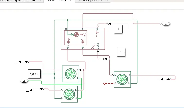
The above figure highlights the vehicle body for electric rickshaw which is having rear axle drive. The Vehicle Body block represents a two-axle vehicle body in longitudinal motion. The block consists of body mass, aerodynamic drag, road incline, and weight distribution between axles due to acceleration and road profile. In optionally we can include pitch and suspension dynamics.

In a vehicle body block

I. NR: It is a physical signal output which is connected to the rear wheel axe!. For this model, it is connected with a normal force of rear tire. 2. NF: It is a physical signal output which is connected to front-wheel axel and for this particular model it is connected with the normal force acting on a front-wheel tire.

3. Beta: Beta is basically a road incline angle. Here we can define a constant value for road angle inclination.

4. H: This port is a horizontal motion of the vehicle body. This connection will be connected with all four Hub of the wheel for finding the thrust generated by the tire.

5. V: This port is the vehicle longitudinal velocity.

6. W: It is a headwind speed. Basically, we will define a particular wind speed by adding constant block.

The Tire (Magic Formula) block models a tire with longitudinal behaviour given by the Magic Formula, an empirical equation based on four fitting coefficients. The block can model tire dynamics under constant or variable pavement conditions.
The Tire (Magic Formula) block models the tire as a rigid wheel-tire combination in contact with the road and subject to slip. When torque is applied to the wheel axle, the tire pushes on the ground (while subject to contact friction) and transfers the resulting reaction as a force back on the wheel. This action pushes the wheel forward or backwards. If you include the optional tire compliance, the tire also flexibly deforms under load. The figure shows the forces acting on the tire.

Battery package modelling:

block used: Battery, powergui, current controlled source, bus selector

Controlled Current Source
The Controlled Current Source block converts the Simulink input signal into an equivalent current source. The generated current is driven by the input signal of the block. The positive current direction is as shown by the arrow in the block icon.
We can initialize the Controlled Current Source block with a specific AC or DC current. If we want to start the simulation in steady state, the block input must be connected to a signal starting as a sinusoidal or DC waveform corresponding to the initial values.

• Double click controlled current source and from drop down menu of measurement select current.

• Signal output will connect with scope by adding current signal to it.

• (+) terminal will connect with battery (-) terminal.

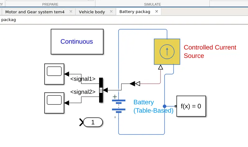
Battery The Battery block implements a generic dynamic model that represents most popular types of rechargeable batteries.
• In battery setup just do the above changes which I highlighted above.

• Just connect ambient temperature with Ta input of battery.

• "M" will be connected with BUS selector lock.

BUS Selector
The Bus Selector block outputs the signals you select from the input bus. The block can output the selected elements separately or in a new virtual bus. • Here just we have mange the output and connect with different Scope Block.

PowerGUI
The powergui block allows us to choose one of these methods to solve your circuit:

• Continuous, which uses a variable-step solver from Simulink

• Discretization of the electrical system for a solution at fixed time steps

• Continuous or discrete phasor solution
The powergui block also opens tools for steady-state and simulation results analysis and for advanced parameter design.

Motor and Gear system:
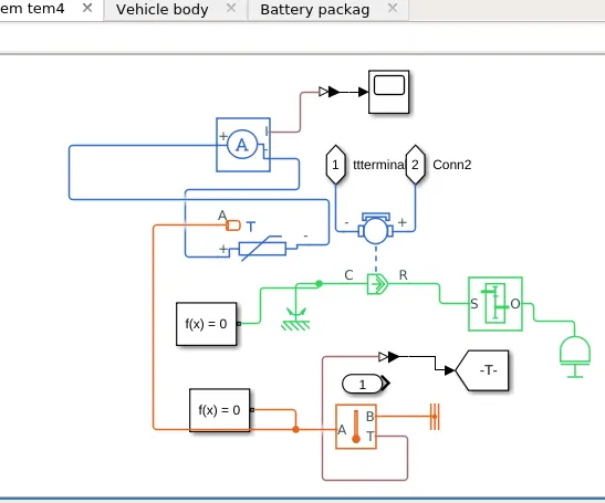
The DC Motor block represents the electrical and torque characteristics of a DC motor using the following equivalent circuit model:
Here in this system, the positive terminal is connected with the current sensor negative terminal and negative terminal is connected with the negative terminal of H-Bridge. R is DC motor rotor which connected with mechanical rotational port i.e. simple gear whereas C is DC motor case and it is connected with mechanical rotational reference.

Driver:
This subsystem compares the input speed and the vehicle speed. If the output is positive speed accelerating command is given from the controller. If the output is negative, deceleration command is given from the controller output. This output is controlled by saturation blocks by giving the upper and lower limits.

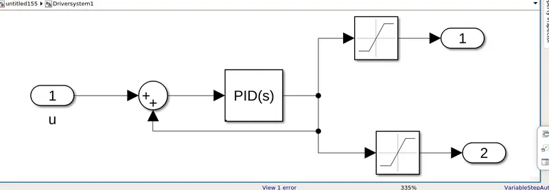
The PID controller is tuned and is a continuous time based.

Power controller:

Simulation mode and Load Assumption Settings

• Power Supply: The power supply is default mode i.e. Internal.

• Simulation Mode: Here I selected Averaged mode and this mode has two Load current characteristics options:

Unsmoothed or discontinuous

• Regenerative Braking: Always enabled (suitable for linearization), this option can be used when the controller always sets the REV flag to ensure regenerative braking.

• Load Current Characteristics: Smoothed, it's a default option and it assumes that the current is practically continuous due to load inductance.

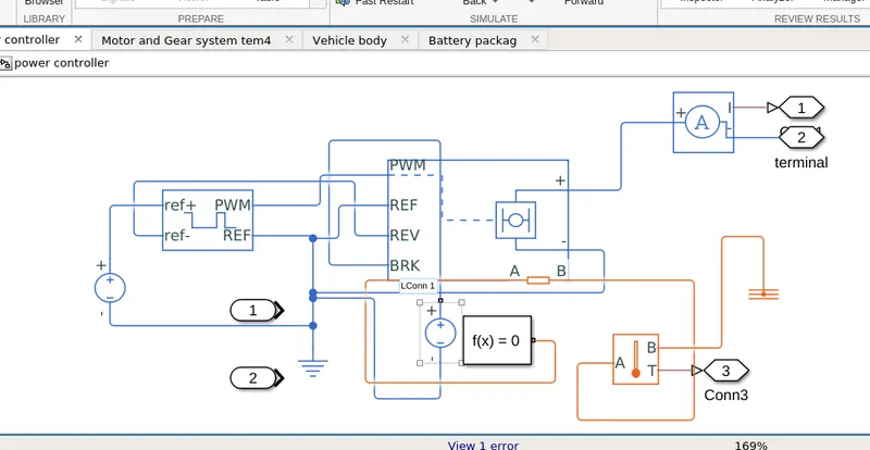
Input Thresholds

• Enable threshold voltage: 1.5 V, this is the above value of PWM at which H-Bridge start.

• PWM signal amplitude: 5.0 V, this is the amplitude of the signal at the PWM input Here I used it as the default node.

• Reverse threshold voltage: 1.5 V, here I changed this value.

• Braking threshold voltage: 2.5 V

Bridge Parameters

• Output voltage amplitude: 60.8 V, this parameter will be active only when we select Internal for Power Supply mode and its an amplitude of the voltage across the H-Bridge.

• Total bridge on resistance: 0.1 ohms,

• The freewheeling diode on resistance: 0.05 ohm

• Measurement Temperature: 25 degC

Temperature Dependency

• Total bridge on resistance at second measurement temperature:00001 ohm

• Freewheeling diode on resistance at second measurement temperature: 001 ohm

• Second measurement temperature:l5 degC

Thermal Port
• Thermal mass: 20000 J/k

• Initial temperature: 25 degC

Detail about connection
• PWM: Pulse-width modulated signal.

• REF: Reference, it is on electrical conversing port associated with the floating zero volts.

• REV: Reverse, it is an electrical conserving port associated with the voltage that controls when to reverse the polarity of the H-Bridge block output.

• BRK: BRK, it is an electrical conserving port associated with the voltage that controls when to short circuit the H-Bridge block output.
Here PWM output port is connected with PWM input port of controlled PWM voltage. The REF and REV port ore connected with REF port of controlled PWM voltage port. The BRK port is connected with a controlled voltage source. The positive (+) terminal is connected with the positive (+) port of current sensor and negative (-) port is connected with the negative (-) port of DC motor. Thermal port (H) is connected with temperature sensor to measure the temperature of controller. CONTROLLED PWM VOLTAGE
ref+ PWM ref- REF
The Controlled PWM Voltage block represents a pulse-width modulated (PWM) voltage source. The input detail is as given below.

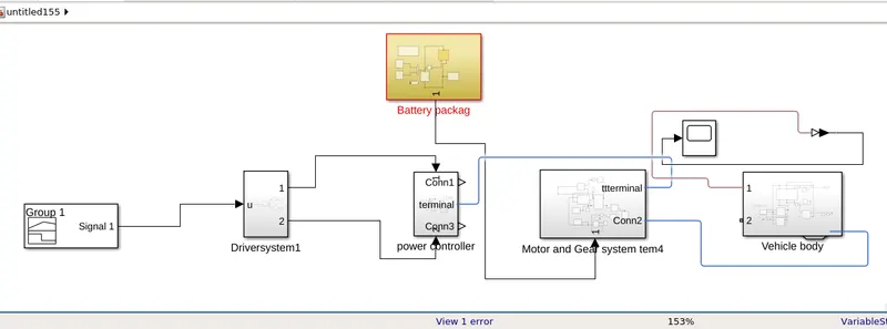
block diagram of electric rickshaw:

RESULTS;

Controller temperature: Temperature of controller rises when the vehicle is running and is constant when it stops. Rise in Temperature is negligible.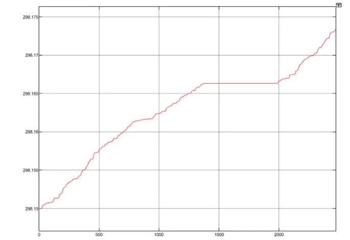

Motor temperature: Motor temperature is increased by 100 deg. K when in operation.This rise of temperature is very high and need to be controlled. It can be concluded that cooling medium is necessary for this powertrain for efficient working and durability.