Final Project: Electric Rickshaw modelling

ELECTRIC RICKSHAW - SYSTEM LEVEL MODELLING

AIM:

To Create a detailed MATLAB model of an electric rickshaw (three wheel passenger vehicle).

OBJECTIVES:

• Rear wheels driven by PM brushed type motor.

• Assume efficiency points of motor controller and motor.

• Make an excel sheet of all input and assumed data.

• For Results any three standard driving cycles show energy consumption, temperature rise of motor and controller for 100 km constant speed driving at 45 kmph.

TO BEGIN WITH:

• Electric rickshaws have been becoming more popular in some cities since 2008 as an alternative to auto rickshaws and pulled rickshaws because of their low fuel cost, and less human effort compared to pulled rickshaws.
• They are being widely accepted as an alternative to petrol/diesel/CNG auto rickshaws.
• They are three-wheelers powered by an electric motor ranging from 650 to 1400 Watts. They are mostly manufactured in India and China.
• Battery-run rickshaws could be a low-emitter complementary transport for the low-income people, who suffer most from a lack of transport facility, if introduced in a systematic manner according to experts.

DESIGN AND CONTRUCTION:

• These rickshaws have a M.S(Mild Steel) tubular Chassis, consisting of three wheels with a differential mechanism at the rear wheels.
• The motor is brushless DC motor manufactured mostly in India and China.
• The electrical system used in Indian version is 48V and Bangladesh is 60V. The body design from most popular Chinese version is of very thin iron or aluminum sheets.
• Vehicles made in fiber are also popular because of their strength and durability, resulting in low maintenance, especially in India.
• Body design is varied from load carriers, passenger vehicles with no roof, to full body with windshield for drivers comfort.
• It consist of a controller unit.They are sold on the basis of voltage supplied and current output, also the number of mosfet (metal oxide field effect transistors) used.
• The battery used is mostly lead acid battery with life of 6–12 months.
• Deep cycle batteries designed for electric vehicles are rarely used.
• Weight of the electric car has also been a recurring design difficulty in them.

MAHINDRA TREO:

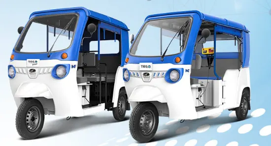
• In Nov 2018, Mahindra Electric launched the Treo range of three-wheelers, powered by Lithium-ion technology.
• The range consists of the Treo, electric auto and Treo Yaari, electric rickshaw.
• The Treo auto boasts an ARAI-certified driving range of 170 km and has a typical driving range of 130 km on the Mahindra Treo after 3 hours 50 minutes of charging.
• The certified range on the Treo Yaari is 130 km that can hit a typical driving range of 85 km after 2 hours 30 minutes of charging.
• Both have a direct drive transmission type, and the Treo has a peak power of 5.4 kW and a peak torque of 30 Nm.
• The Treo Yaari has a peak power of 1.96 kW and a peak torque of 19 Nm.
• Both the Treo and the Treo Yaari have a wheelbase of 2050 mm and a turning radius of 2.9 m.
• The Treo range has a vehicle kerb weight between 340–350 kg, while the Treo Yaari range has a vehicle kerb weight between 265–275 kg.

MATLAB MODEL:

• Now lets go ahead and prepare a matlab model of an Electric Rickshaw.
• we will be modelling in a way where the model Achieves the given Objectives.

BASIC BLOCK DIAGRAM:

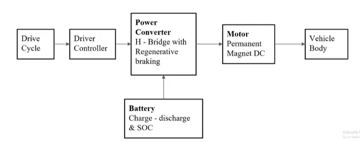
• in the designed Electric Rickshaw main blocks are the Battery, Drive cycle, controller, DC motor, Vehicle body and Transmission system.
• Drive cycle is the input data like how a human drive his actual.
• We will be using 3 drive cycles.
  
  • User defined drive cycle.
  • Urban Dynamometer Driving Schedule (UDDS) driving cycle,
  • The Highway fuel economy test (HWFET).
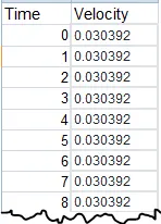
• there drive cycles are manually prepared in Excel sheet, to make the designed vehicle to give the output how it reacts to the drive cycle.
• The main objective is to obtain the speed by the driver, to estimate the temperature of motor and controller, to estimate the state of Charge (SOC), distance travelled by the vehicle.

SIMULINK MODEL:

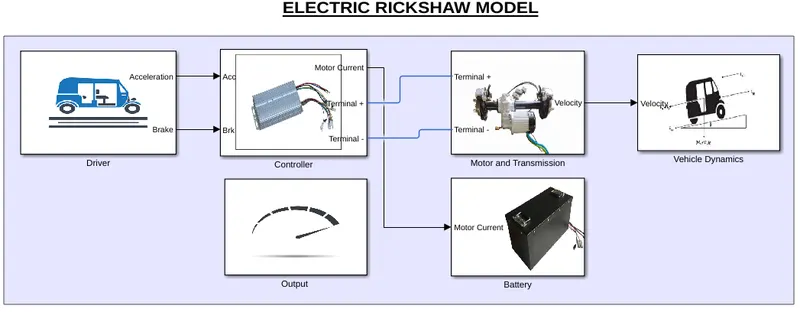
• This is a model representing the Electric Rickshaw, where we have all the block performing individual operations.
• we have arranged the blocks as per their functions in a subsystem fashion.
• the input is delivered from the Driver where we will be using drive cycles, and producing output as Acceleration and Braking.
• with Acceleration and braking the output is fed as input to the controller, where the controller uses PWM and H-Bridge for regulating the control signal.
• the controller is connected to the motor and transmission system and also supplies current to the battery and also consumes energy from battery.
• the Distance will be calculated in the Vehicle dynamics system and output will be displayed in the output block.
• now, lets discuss each and every systems briefly.

Driver:

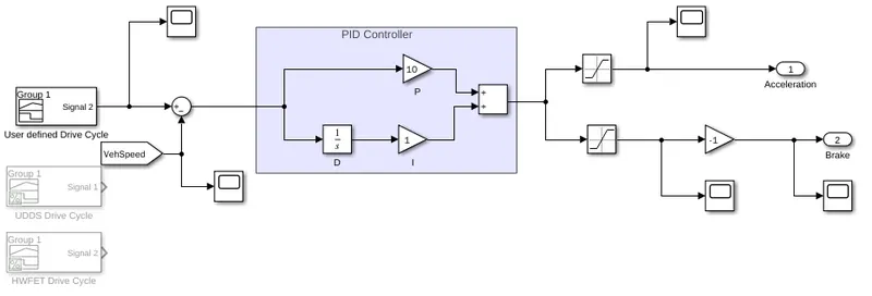
• the drive cycles produce the input speed.
• the drive cycles are customized with the singal builder block.
• this system compares the input speed and the vehicle speed using the sum block.
• If the output is positive speed acceleration is given from the PI controller, and the negative output, deceleration is also given from the controlled.
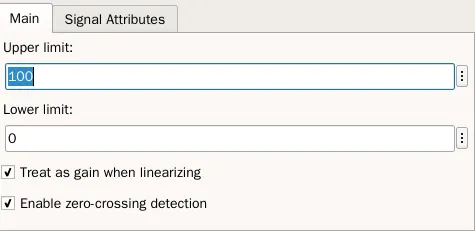
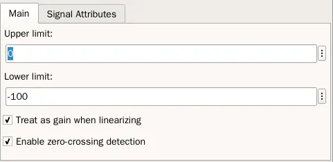
• The output from the controller is controlled by the saturation blocks by given the upper and lower limits.
• we have kp as 10 and ki as 1, and it tuned in a continuous time based.
• inorder to send the braking in negative we are using a Negative to multiply with the help of gain block.

Drive Cycle:

• Drive cycle is assumed as the driver's input of a vehicle.
• It is the Data representing the driving condition of a driver.
• these drive cycles will have high-speed, low-speed and braking conditions.
• as dicussed above will be using three different drive cycles.
• all these drive cycles will be generating signals from the singal builder block.

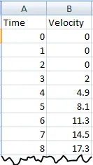
1. User Defined Drive Cycle:

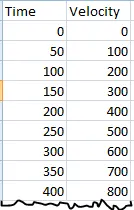
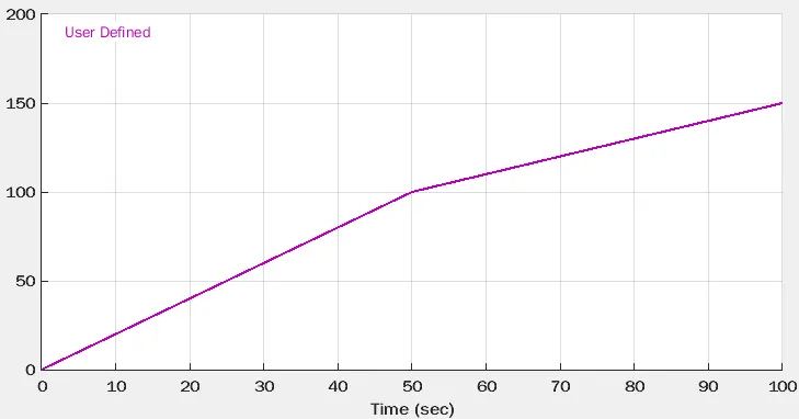
• This drive cycle was defined by me, where there is no braking and velocity will be increasing as time increases.
• we have initial velocity as 0 and velocity increases with respect to time.

2. Urban Driving Drive Cycle (UDDS):

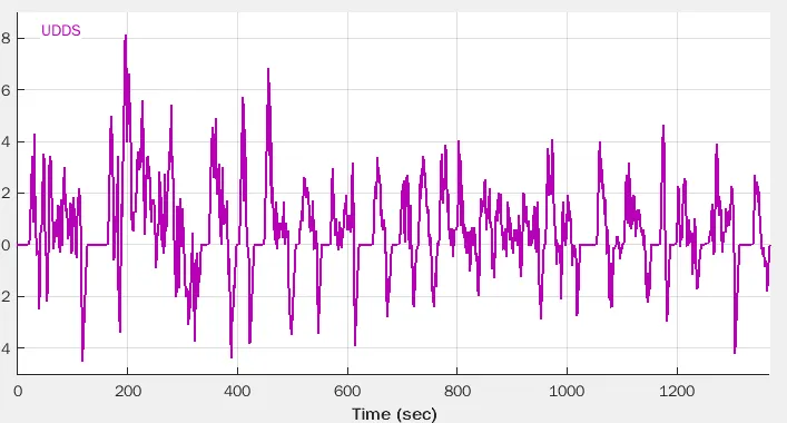
• The ECE is an urban driving cycle, also known as UDC.
• It was devised to represent city driving conditions, e.g. in Paris or Rome.
• It is characterized by low vehicle speed, low engine load, and low exhaust gas temperature.
• The cycle simulates a urban route of 7.5 mi (12.07 km) with frequent stops.
• The maximum speed is 56.7 mph (91.25 km/h) and the average speed is 19.6 mph (31.5 km/h).

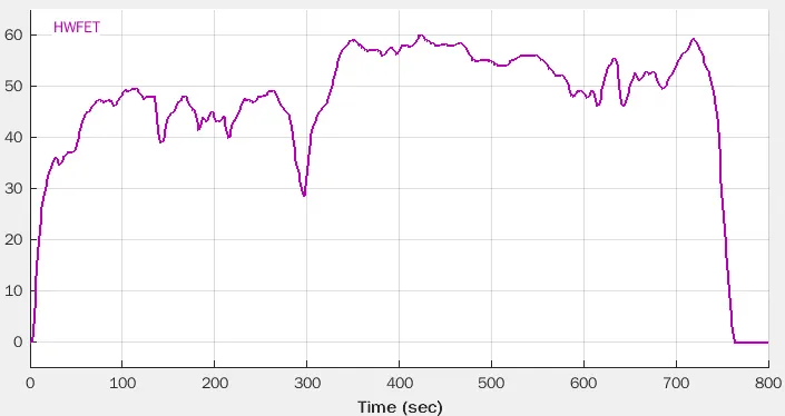
3. The Highway fuel economy test (HWFET):

• The Highway Fuel Economy Test (HWFET or HFET) cycle is a chassis dynamometer driving schedule.
• it was developed by the US EPA for the determination of fuel economy of light duty vehicles [40 CFR 600, subpart B] .
• The HWFET is used to determine the highway fuel economy rating, while the city rating is based on the FTP-75 test.

Saturation block parameters:

• Limit input signal to the upper and lower saturation values.

CONTROLLER:

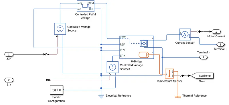
• the output from the driver block i.e. Acceleration and brake is given as the input for the controller.
• controller is one of the main components of the Electric Rickshaw that governs it's complete operation.
• lets dicuss the block configurations.,

Blocks Used:

• Controlled voltage source converts a Simulink input signal into an equivalent voltage source.
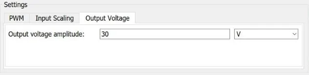
• The Controlled PWM Voltage block represents a pulse-width modulated (PWM) voltage source.
• The H-Bridge block represents an H-bridge motor driver,The H-Bridge block output is a controlled voltage that depends on the input signal at the PWM port.
• The Current Sensor block represents an ideal current sensor, that is, a device that converts current measured in any electrical branch into a physical signal proportional to the current.
• The Temperature Sensor block represents an ideal temperature sensor, that is, a device that determines the temperature differential measured between two points without drawing any heat.
• The Solver Configuration block specifies the solver parameters that your model needs before you can begin simulation.
• The Electrical Reference block represents an electrical ground. Electrical conserving ports of all the blocks that are directly connected to ground must be connected to an Electrical Reference block. A model with electrical elements must contain at least one Electrical Reference block.
• The Thermal Reference block represents a thermal reference point, that is, a point with an absolute zero temperature, with respect to which all the temperatures in the system are determined.

Settings made inside the blocks:

Double tap on the Block to make the respective changes:

• H-Bridge block: Enable the thermal port of the block by right clicking on the block and select simscape>block choice>thermal port.

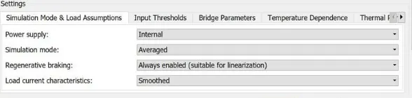
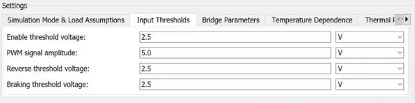
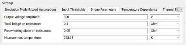
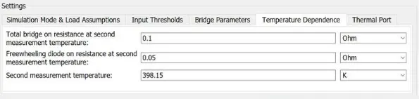
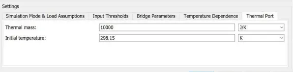
• Controlled PWM Voltage Block:

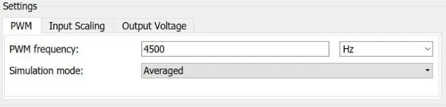
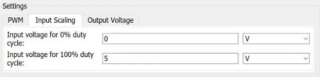
MOTOR AND TRANMISSION:

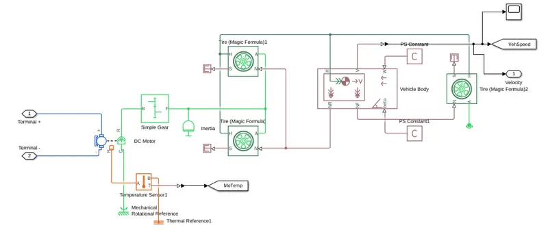
• the H-Bridge's positive and Negative terminal is supplied as input for the DC motor.
• the rotor of the DC motor is connected to the Gear Box, and for speed compounding we are using Interia.
• the hub of the tire is connected to the Vehicle hub and the S is been terminated.
• the wind and terrain is supplied with ps contact block.
• and we are getting output as Vehicle speed.

Blocks Used:

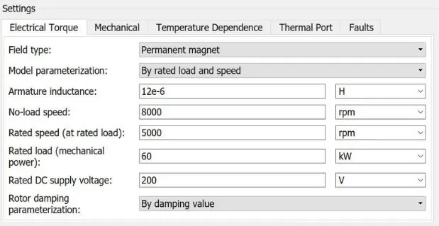
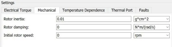
• The DC Motor block represents the electrical and torque characteristics of a DC motor.
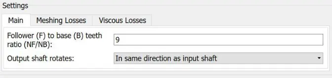
• The Simple Gear block represents a gearbox that constrains the connected driveline axes of the base gear, B, and the follower gear, F, to corotate with a fixed ratio that you specify.
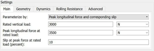
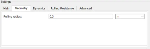
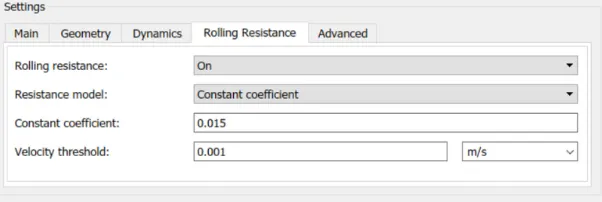
• The Tire (Magic Formula) block models a tire with longitudinal behavior given by the Magic Formula, an empirical equation based on four fitting coefficients. The block can model tire dynamics under constant or variable pavement conditions.
• The longitudinal direction of the tire is the same as its direction of motion as it rolls on pavement. This block is a structural component based on the Tire-Road Interaction (Magic Formula) block.
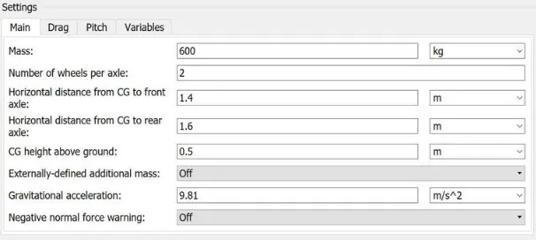
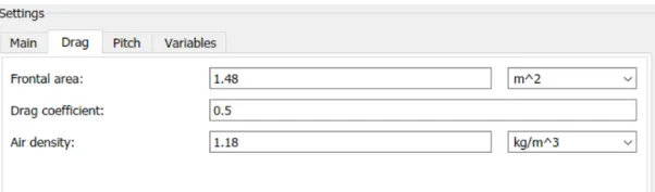
• The Vehicle Body block represents a two-axle vehicle body in longitudinal motion. The vehicle can have the same or a different number of wheels on each axle. For example, two wheels on the front axle and one wheel on the rear axle. The vehicle wheels are assumed identical in size. The vehicle can also have a center of gravity (CG) that is at or below the plane of travel.
• The Temperature Sensor block represents an ideal temperature sensor, that is, a device that determines the temperature differential measured between two points without drawing any heat.
• The Mechanical Rotational Reference block represents a reference point, or frame, for all mechanical rotational ports. All rotational ports that are rigidly clamped to the frame (ground) must be connected to a Mechanical Rotational Reference block.

Settings made inside the blocks:

Double tap on the Block to make the respective changes.

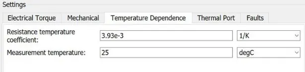
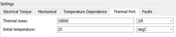
• DC Motor:

• Tire Block:

• Gear:

• Vehicle Body:

BATTERY:

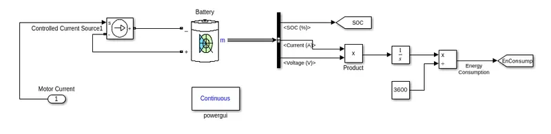
• the input for the battery is from the motor current from the controller block.
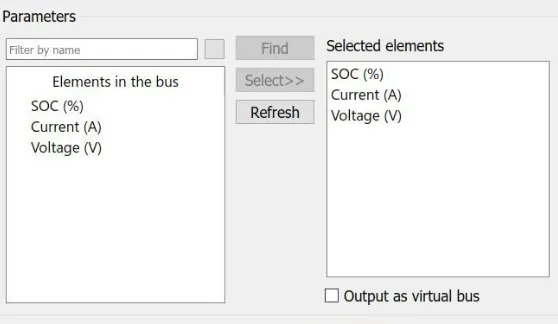
• the current source is connected to the battery and we are using a bus selector to find the SOC, Current and voltage.
• but mulitplying current and voltage, the product is intergated and given as Energy Consumped.

Blocks Used:

• The Controlled Current Source block converts the Simulink input signal into an equivalent current source. The generated current is driven by the input signal of the block. The positive current direction is as shown by the arrow in the block icon.
• The Battery block implements a generic dynamic model that represents most popular types of rechargeable batteries.
• The Bus Selector block outputs the elements you select from the input bus. The block can output the selected elements separately or in a new virtual bus.
• The Product block outputs the result of multiplying two inputs: two scalars, a scalar and a nonscalar, or two nonscalars that have the same dimensions.
• The Integrator block outputs the value of the integral of its input signal with respect to time.
• The Divide block outputs the result of dividing its first input by its second. The inputs can be scalars, a scalar and a nonscalar, or two nonscalars that have the same dimensions. This block supports only complex input values at division ports when all ports have the same single or double data type.

Settings made inside the blocks:

Double tap on the Block to make the respective changes.

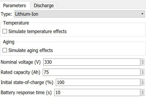
• Battery:

• Bus Selector:

VEHICLE DYNAMICS:

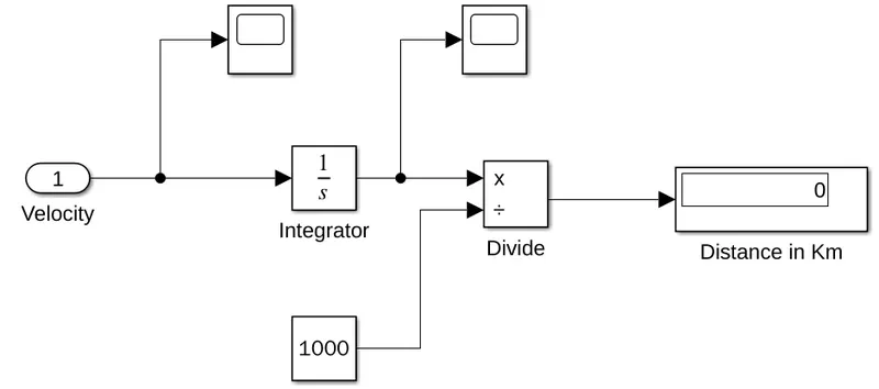
• In the Vehicle dynamics block we will be calculating the Distance travelled by the Vehicle.
• we know that the Distance is obatined by Intergating Velocity.
• the Distance will be displayed in the display block.
• for meter to kilo meter conversion we are dividing Velocity in m with 1000 to get Km.

OUTPUT (block):

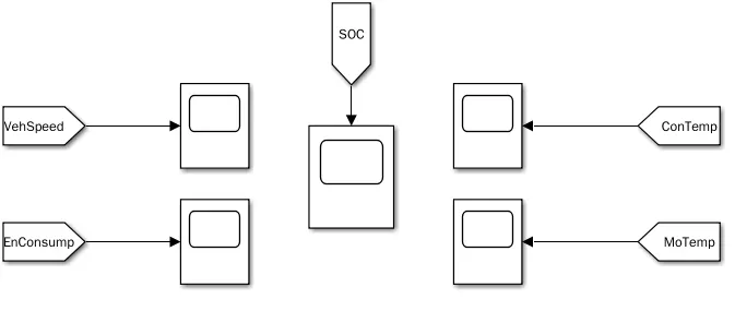
• the output is from the output block.
• here we have from tags from respective Gotos' to represent the output.
• scope blocks are used to screen the output.
• we can get the Vehicle speed, Energy consumption, SOC, and rising temperature of controller and Motor from this block.

OUTPUT:

• Now lets run the system.
• At first we will connect the user defined driving cycle and check for results.
• after simultion of that drive cycle we will switch on to the next Drive Cycle:

Output - User Defined Drive Cycle:

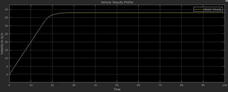
• from the velocity profile graph we can understand the characteristics of Vehicle Velocity.
• we can see that the velocity depends on the Drive cycle which we provided as an Input.
• the inital velocity as 0 m/s at 0 s, and gradually increases to 36 m/s at 20 s.
• the velocity saturates at 37 m/s and travells throught the time.

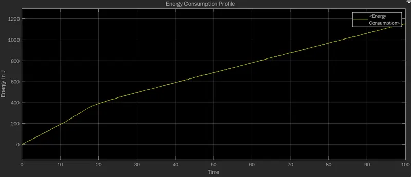
• from the energy consumption profile we can understand the energy consumption of the system.
• the energy is consumped as per the drive cycle we gave as an input.
• the 0 energy is consumed at 0 s, and when time increases the energy increase along with it.
• the energy consumed at 20 s is 400 J and keep on increasing as time increases.

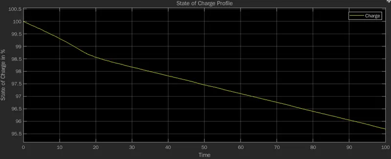
• From the SOC profile graph we can understand the charging level.
• the vehicle starts at 100 % charge and reduces to 95 percentage in 100 s.
• since there is no braking involved the battery gets charged on the go, resulting in good battery percentage.

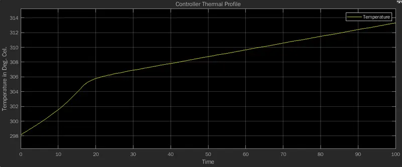
• the controller thermal profile graph explains us the Rise/Fall in temperature of the Controller.
• we can see the initial temperature is 298 dc and increases as time increases.

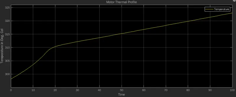
• the Motor thermal profile graph explains us the Rise/Fall in temperature of the Controller.
• we can see the initial temperature is 298 dc and increases as time increases.
• the motor and controller temperature seems similair in both graphs.

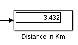
• as per the Given drive cycle, we can understand the distance travelled is 3.4 km for 100 s.

Output - User Defined Drive Cycle:

let us now change the drive cycle from user defined to UDDS, and observe the output.

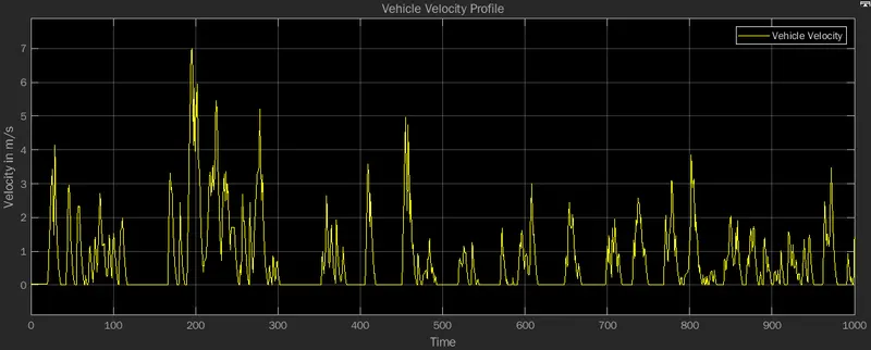
• from the velocity profile graph we can understand the characteristics of Vehicle Velocity.
• we can see that the velocity depends on the Drive cycle which we provided as an Input.
• the inital velocity as 0 m/s at 0 s.
• we can see there is lot of acceleration and decceleration involved, which produces spikes in out graph.
• the peak response it at 7 m/s at 200 sec.
• so the velocity sticks with the drive cycle.

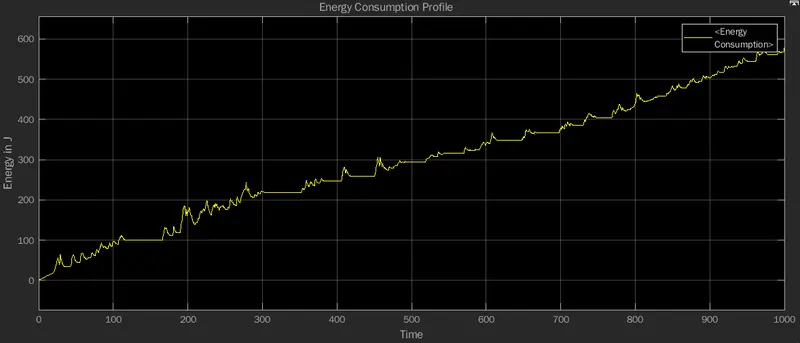
• from the energy consumption profile we can understand the energy consumption of the system.
• the energy is consumped as per the drive cycle we gave as an input.
• the 0 energy is consumed at 0 s, and when time increases the energy increase along with it.
• with comparing with the previous graph we can see uneven rising and falling in the Graph.
• that is because of the drive cycle values we have given as input.
• and redistribution of energy occurs due to the regenerative braking.

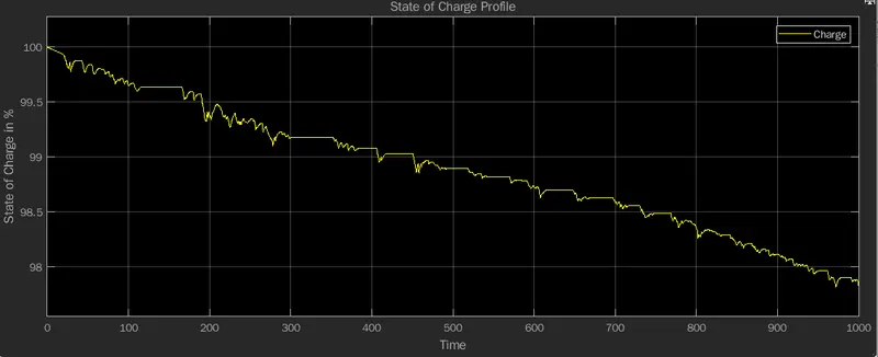
• From the SOC profile graph we can understand the charging level.
• the vehicle starts at 100 % charge and reduces to 98 percentage in 1000 s.
• since there is acceleration/decceleration involved, the battery gets charged as the vehicle deccelerates.
• this Drive cycle is more efficient than compared to the previous drive cycle.

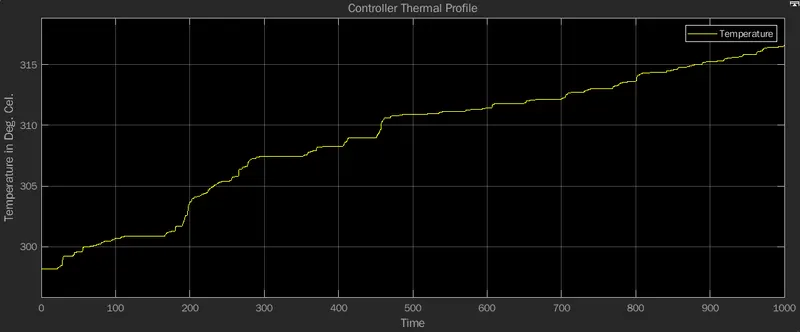
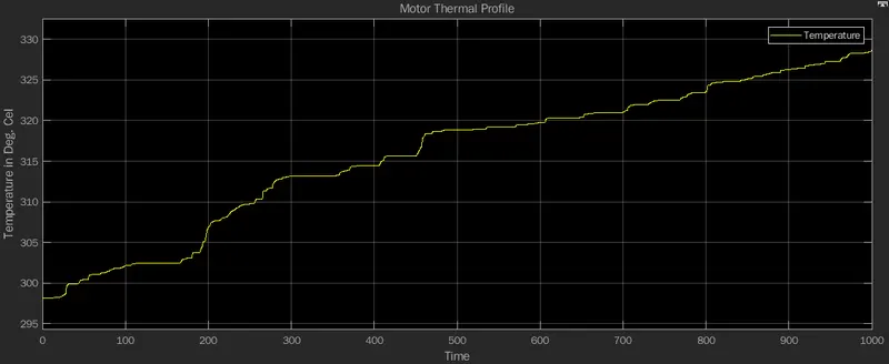
• the motor and controller thermal profile tells us the Rise/Fall in temperature inside the Motor and controller.
• as we can see the both system starts thier temp as 298 dc and increases as time increases.
• there is rise and fall in the temperature due to acceleration/deceleration happening in the drive cycle.

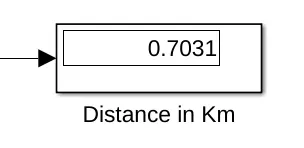
• as per the Given drive cycle, we can understand the distance travelled is 0.7 km for 1000 s.

Output - The Highway fuel economy test (HWFET):

let us now change the drive cycle from UDDS to HWFET, and observe the output.

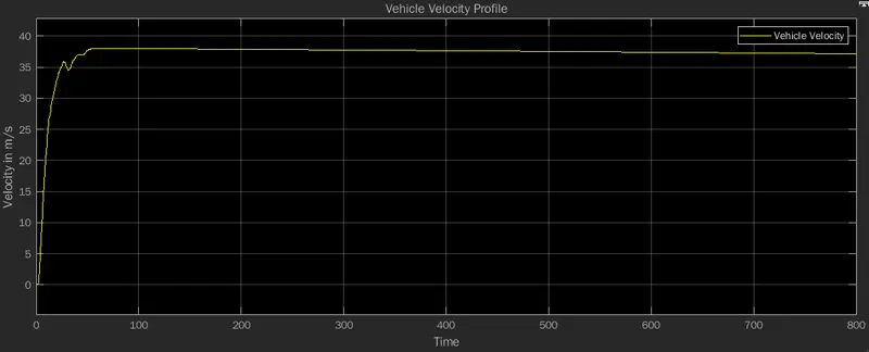
• from the velocity profile graph we can understand the characteristics of Vehicle Velocity.
• we can see that the velocity depends on the Drive cycle which we provided as an Input.
• the inital velocity as 0 m/s at 0 s, and gradually increases to 36 m/s at 20 s.
• there is small decelleration at 30s which changes the rate of veolocity.
• the velocity saturates at 37 m/s and travells throught the time.

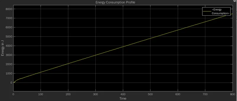
• from the energy consumption profile we can understand the energy consumption of the system.
• the energy is consumped as per the drive cycle we gave as an input.
• the 0 energy is consumed at 0 s, and when time increases the energy increase along with it.
• the energy consumed keep on increasing as time increases.

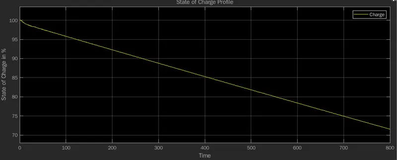
• From the SOC profile graph we can understand the charging level.
• the vehicle starts at 100 % charge and reduces to 95 percentage in 100 s.
• at the end of Course the Charge level is 70 %.

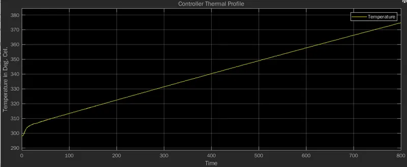
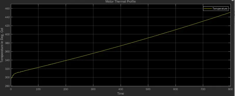
• the motor and controller thermal profile tells us the Rise/Fall in temperature inside the Motor and controller.
• as we can see the both system starts thier temp as 298 dc and increases as time increases.
• since the vehicle operates in constant speed and increases as time increases.

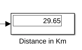
• as per the Given drive cycle, we can understand the distance travelled is 30 km for 800 s.

COMPARISON:

• now lets compare the three driving cycles with respect to Velocity, Energy consumption, Temperatures of motor and controller and State of Charge.
• in contrast with Velocity HWFET is better compared with Us.De.D.S and UDDS as the velocity is 37 m/s.
• for Energy consumption UDDS is better than HWFET and Us.De.D.S as it consumes 550 J for 1000 s.
• in Thermal conditions all three Drive cycles performed well.
• for SOC we can see that UDDS starts at 100 and only 2 % of charge consumed for 1000 s.

CONCLUSION:

• Thus the Electric rickshaw driven by PM brushed type motor has been modelled using MATLAB successfully.
• Thus the Results For three standard driving cycles is obtained.
• The energy consumption, temperature rise of motor and controller, Vehicle speed and SOC has been determined.

POPULARITY IN INDIA:

• One of the first attempts to design electric rickshaws was done by Nimbkar Agricultural Research Institute in late 1990s.
• In India, these so-called e-rickshaws are widely spread all over the country, starting to gain popularity around 2011.
• The design is now much different from cycle rickshaws.
• Today, e-rickshaws play a vital role in providing livelihood to people in India.
• Due to their low cost and high efficiency they are accepted on the Indian streets, but government policies have been threatening the e-rickshaw and banned its use in the capital city Delhi,but failed to put them off the streets.
• E-rickshaws are still rising in number and widely used in Delhi and other parts of India.
• In Delhi, as per government official's figures in April 2012, their number was over 100,000.

ELECTRIC RICKSHAW LAW IN INDIA:

• Initially e-rickshaws were unregulated by any central law in India.
• However, the Delhi High Court, banned running of e-rickshaws in Delhi on 31 July 2014, over safety concerns raised through a public interest litigation.
• In a rally held for regularization of e rickshaws in Delhi transport minister Nitin Gadkari said that "municipal corporations would regularize e-rickshaws by registering them for a fee of just ₹100.
• After registering the e-rickshaw, corporations will have to issue identity cards to drivers so they can earn their livelihood easily.
• Once the policy was in place, the corporation, along with traffic police, would have fix the amount of fine to be imposed for violation of the policy.
• However, the policy was never implemented.
• Certain states like Tripura had regularised the e-rickshaws through municipal bylaws or through state legislation.
• In March 2015, the Indian Parliament passed an amendment to the Motor Vehicles (Amendment) Bill, 2015 legalizing e-rickshaws.
• By July 2015, battery rickshaws are available for travel in many cities, now certified to ply with Registration No. plate by R.T.O. with insurance.

TOP 10 E RICKSHAW MANUFACTURERS IN INDIA:

1. Mahindra E Rickshaw
2. Mayuri e-Rickshaw
3. Jezza Motors
4. Udaan vehicles
5. Thukral e rickshaw
6. Vidhyut E-Rickshaw
7. Big Bull E-rickshaw
8. Bahubali e-Rickshaw
9. Goenka e-rickshaw (GEM e-rickshaw)
10. Queen e-Rickshaw.

FROM THE NEWS:

• Oye Rickshaw plans to deploy over one lakh e-rickshaws this year, expand ops to 25 new cities. January 12, 2022.
• Honda to establish subsidiary in India for e-rickshaw battery sharing service, October 30, 2021.
• Electric Vehicle City to charge up Uttar Pradesh's e-rickshaw manufacturing units September 6, 2021.
• Gurgaon's e-rickshaw zones identified, rollout plan soon August 4, 2021 .
• MCG plans Rs 30,000 subsidy to drivers for e-rickshaw rollout, April 8, 2021.

RESULT:

Thus the Project is completed successfully and output is verifed.