Final Project: Electric Rickshaw modelling
Create a detailed MATLAB model of an electric rickshaw (three wheel passenger vehicle) as per details below:
Rear wheels driven by PM brushed type motor
Assume efficiency points of motor controller and motor
Make an excel sheet of all input and assumed data
Results: For any three standard driving cycles show energy consumption, temperature rise of motor and controller for 100 km constant speed driving at 45 kmph.
Create a MATLAB model of electric car which uses lithium ion battery and suitable motor. Choose suitable blocks from Simscape or Powertrain block set. Implement the vehicle speed control using PI controller and generate brake and accelerator commands. Avoid using readymade driver block for speed control.
Prepare a report about your model including following:
Objectives, System level configurations, Model parameters, Results, Conclusion.
ANS:
AIM:
To create a detailed MATLAB model of an electric rickshaw (three wheel passanger vehicle)
Objective:
- Rear wheels is driven by PM brushed type motor
- Assuming efficiency points of motor controller and motor
- To create an excel sheet of all input and assumed data
- Temperature rise of motor and controller for 100 km constant speed driving at 45 kmph
- Energy consumption values for any three standard drive cycles
Introduction:
Electric rickshaws (also known as electric tuk-tuks or e-rickshaws or toto or e-tricycles) have been becoming more popular in some cities since 2008 as an alternative to auto rickshaws and pulled rickshaws because of their low fuel cost, and less human effort compared to pulled rickshaws. They are being widely accepted as an alternative to petrol/diesel/CNG auto rickshaws. They are three-wheelers powered by an electric motor ranging from 650 to 1400 Watts. They are mostly manufactured in India and China. Battery-run rickshaws could be a low-emitter complementary transport for the low-income people, who suffer most from a lack of transport facility, if introduced in a systematic manner according to experts.
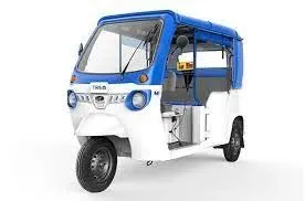
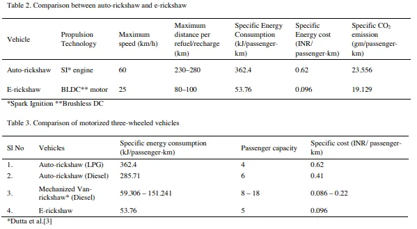
Table 2 shows the comparison between the different parameters for the e-rickshaw and the auto-rickshaw. Compared to all the forms of motorized three-wheeled vehicles, the e-rickshaws were found to be the most energy efficient among the clan, and can be considered for exact replacement of the mechanized van-rickshaws from which the e-rickshaws were technically superior. Table 3 shows the comparison of the specific energy consumption, passenger capacity, and specific cost of transportation among all the motorized three-wheelers.
BLOCK DIAGRAM:
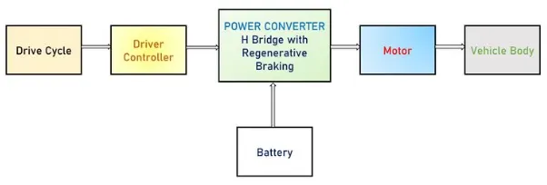
Fig.1 Block digram of an E-rickshaw model
In this block diagram the main blocks are Battery, controller, DC Motor, drive cycle, Vehicle body & Transmission system. Drive cycle is the input data which is a series of data points representing the speed of vehicle Vs time. Here FTP75, Excel (Manually Prepared in Excel sheet) & an user defined cycle drive cycles are used to make designed vehicle to give output how it reacts to the drive cycle. The main objective is to obtain the speed by the driver, to estimate the sates of charge (SOC), to estimate the temperature of Motor and Controller, distance travelled by the vehicle. The SOC block in the model will estimate the state of charge of a battery, distance is calculated by speed and time parameters for all the three Drive cycles.
MATLAB model of an Electric Rickshaw:
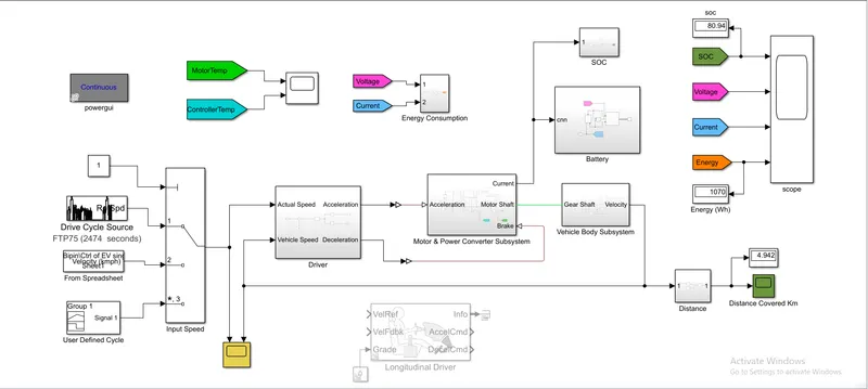
Now let us discuss each of the blocks used to create this MATLAB model.
Detailed Study of Model Parameters:
DRIVE CYCLE
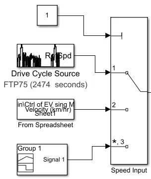
Drive cycle is simply a speed vs time graph which is assumed as driver's input of a vehicle. Here to test the vehicle performance I have used three drive cycles. These drive cycles consists of low speed, high speed, braking condition etc. on it. Here I have used FTP75, Excel (Manually Prepared in Excel sheet) & an user defined cycle as three standard drive cycles.
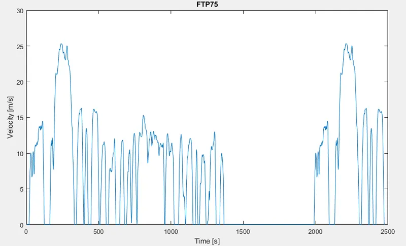
- FTP75 (2474 seconds)
Generates a standard or user-specified longitudinal drive cycle. The block output is the vehicle longitudinal speed. The drive cycle was simulated for 2474 seconds.
- Wide open Throttle (WOT) (60 seconds)
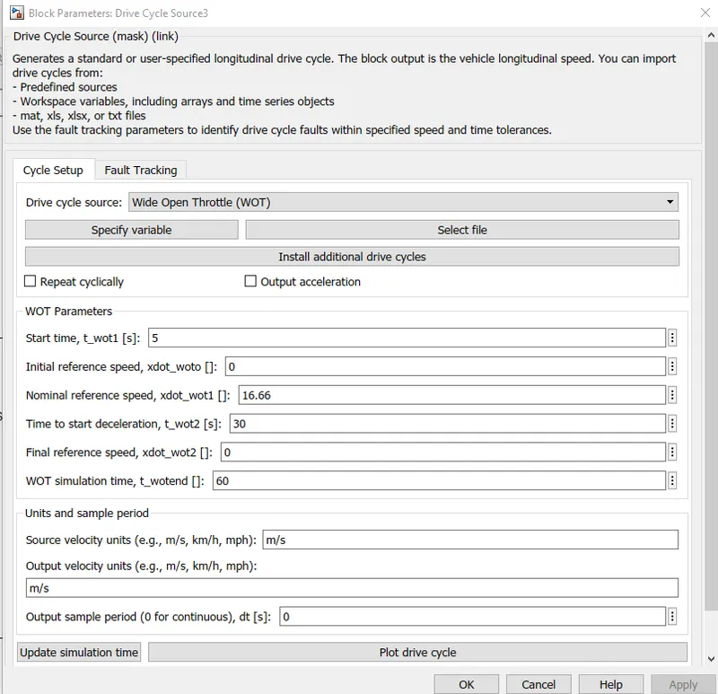
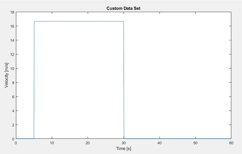
WOT drive cycle is of 60 seconds where the signal starts at 5 seconds & starts decelerating after 30 seconds.
- User Defined Drive Cycle
This cycle has a constant speed of 45kmph or 12.5m/s for 8000 seconds. The reason of the time being 8000 seconds is that the vehicle will take 8000 seconds for completing 100km ride at 45kmph speed.
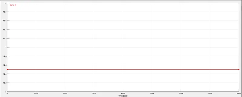
To create a user defined cycle having constant speed driving @45 kmph for 100 kms run & 8000 seconds using signal builder block.
Speed= Distance/Time
Time= Distanced/Speed
`therefore(100km)/(45 kmph)`
`=2.222222 hr`
Hours to second conversion:
`2.22222times3600`
`=7999.999 approx 8000 seconds`
Converting 45 kmph into m/s gives `45times(1000/3600)=12.5ms^-1`
These inputs are fed into signal builder block to create an user defined drive cycle.
Multiport Switch:
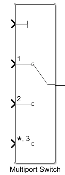
All the three drive cycles are controlled by the controller provided above the Constant through multi-port switch. The Multiport Switch block determines which of several inputs to the block passes to the output. The block bases this decision on the value of the first input. The first input is the control input and the remaining inputs are the data inputs. The value of the control input determines which data input passes to the output.
DRIVER BLOCK:
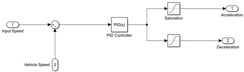
To build an driver subsystem block a PID controller is used. This subsystem compares the input/actual speed and the vehicle speed. These two speeds are given to a sum block. If the error produced is positive speed accelerating command is given by the controller & if it's negative speed decelerating command id given by the controller output. These outputs are controlled by the saturation blocks by providing the upper & lower limits.
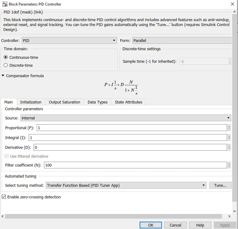
The PID controller is tuned & is of continuous time based.
MOTOR & POWER CONVERTER SUBSYSTEM:
This subsystem has the blocks which are used to create the voltage signals to control the motor speed as per the input drive cycle data.
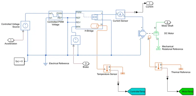
This subsystem is connected to the driver block output ports namely acceleration command and deceleration command.
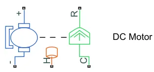
This subsystem converts this acceleration and deceleration command into voltage signals using 2 controlled voltage source block, controlled PWM voltage block, a H-bridge, a current sensor. Temperature sensor block is used to sense the temperature rise in both controller & motor respectively.
Controlled Voltage Source:-
The output voltage is V = Vs, where Vs is the numerical value presented at the physical signal port.
The block has one physical signal input port and two electrical conserving ports associated with its electrical terminals.
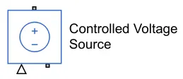
The controlled voltage source block don't have it's own block parameters. It receives input signal from the longitudinal driver block and the output is given to H-bridge block.
Controlled PWM Voltage:-
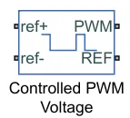
The block creates a Pulse-Width Modulated (PWM) voltage across the REF and REF ports. When the pulse is low the output voltage is zero and when the pulse is high, the output voltage is equal to the Output voltage amplitude parameter. Duty cycle is set by input value.
The Simulation mode can be set to Averaged or PWM. In the PWM mode, the output is a PWM signal. In Averaged mode, the output is a constant with value equal to averaged PWM signal.
PARAMETERS:
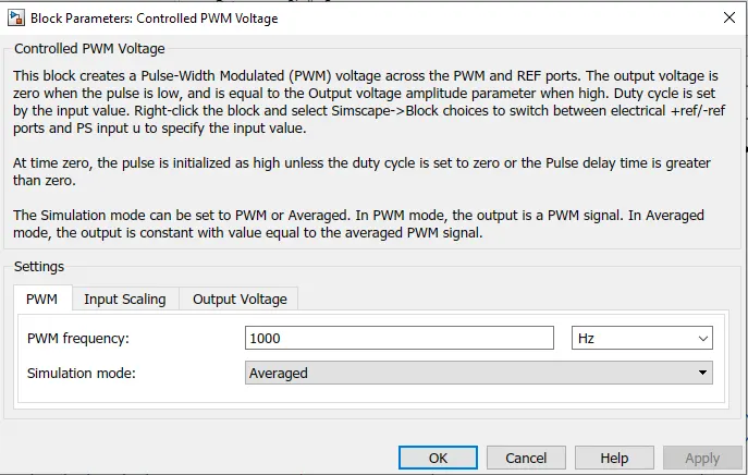
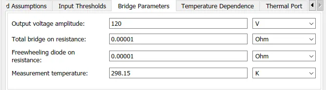
The PWM frequency is set to 1000 Hz and the simulation mode selected is average mode.
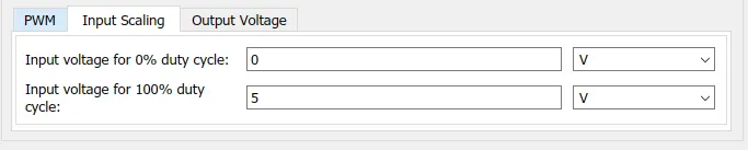
The input voltage for 100% duty cycle is kept as default 5 Volts.

The output voltage amplitude is set for 50 volts for more precise results.
H-Bridge:-
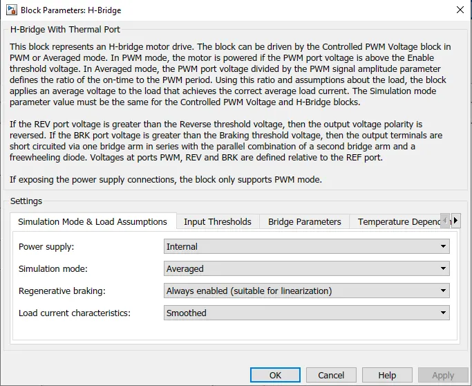
The H-Bridge block represents an H-bridge motor driver. The block has the following two Simulation mode options:
-
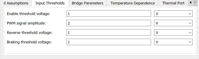
PWM — The H-Bridge block output is a controlled voltage that depends on the input signal at the PWM port. If the input signal has a value greater than the Enable threshold voltage parameter value, the H-Bridge block output is on and has a value equal to the value of the Output voltage amplitude parameter. If it has a value less than the Enable threshold voltage parameter value, the block maintains the load circuit using one of the following three Freewheeling mode options:
- Via one semiconductor switch and one freewheeling diode
- Via two freewheeling diodes
- Via two semiconductor switches and one freewheeling diodeThe first and third options are sometimes referred to as synchronous operation.
The signal at the REV port determines the polarity of the output. If the value of the signal at the REV port is less than the value of the Reverse threshold voltage parameter, the output has positive polarity; otherwise, it has negative polarity.
-
Averaged — This mode has two Load current characteristics options:
1) Smoothed
2) Unsmoothed or discontinuous
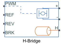
PORTS:
PWM - Input port for PWM voltageREF - Input port for reference PWM voltage
REV - Input port for reverse signal
BRK - Input port for brake signal
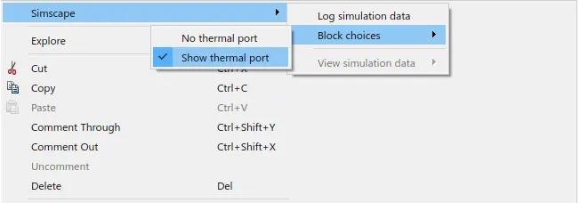

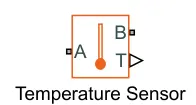
The Temperature Sensor block represents an ideal temperature sensor, that is, a device that determines the temperature differential measured between two points without drawing any heat.
Connections A and B are thermal conserving ports that connect to the two points where temperature is being monitored. Port T is a physical signal port that outputs the temperature differential value.
The block positive direction is from port A to port B. The measured temperature is determined as T = TA – TB.
Electrical Reference:-
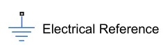
The Electrical Reference block represents an electrical ground. Electrical conserving ports of all the blocks that are directly connected to ground must be connected to an Electrical Reference block. A model with electrical elements must contain at least one Electrical Reference block. The block has one electrical conserving port.
Mechanical Rotational Reference:-
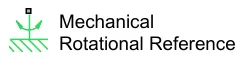
The Mechanical Rotational Reference block represents a reference point, or frame, for all mechanical rotational ports. All rotational ports that are rigidly clamped to the frame (ground) must be connected to a Mechanical Rotational Reference block. The block has one mechanical rotational port.
Thermal Reference:-
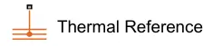
The Thermal Reference block represents a thermal reference point, that is, a point with an absolute zero temperature, with respect to which all the temperatures in the system are determined. The block has one thermal conserving port.
Solver Configuration:-
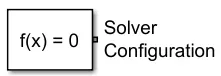
Each physical network represented by a connected Simscape™ block diagram requires solver settings information for simulation. The Solver Configuration block specifies the solver parameters that your model needs before you can begin simulation.
Each topologically distinct Simscape block diagram requires exactly one Solver Configuration block to be connected to it.
VEHICLE DYNAMICS:
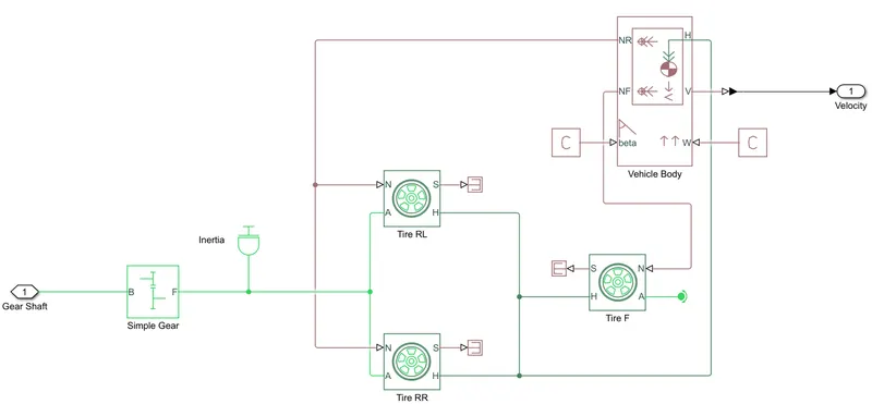
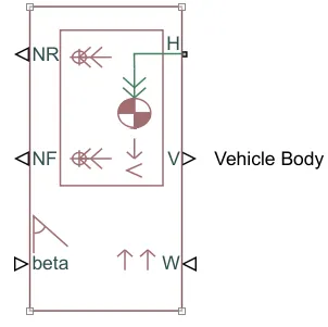
The Vehicle Body block represents a two-axle vehicle body in longitudinal motion. The vehicle can have the same or a different number of wheels on each axle. For example, two wheels on the front axle and one wheel on the rear axle. The vehicle wheels are assumed identical in size. The vehicle can also have a center of gravity (CG) that is at or below the plane of travel.
The block accounts for body mass, aerodynamic drag, road incline, and weight distribution between axles due to acceleration and road profile. Optionally include pitch and suspension dynamics. The vehicle does not move vertically relative to the ground.
The block has an option to include an externally-defined mass and an externally-defined inertia. The mass, inertia, and center of gravity of the vehicle body can vary over the course of simulation in response to system changes.
PARAMETERS:
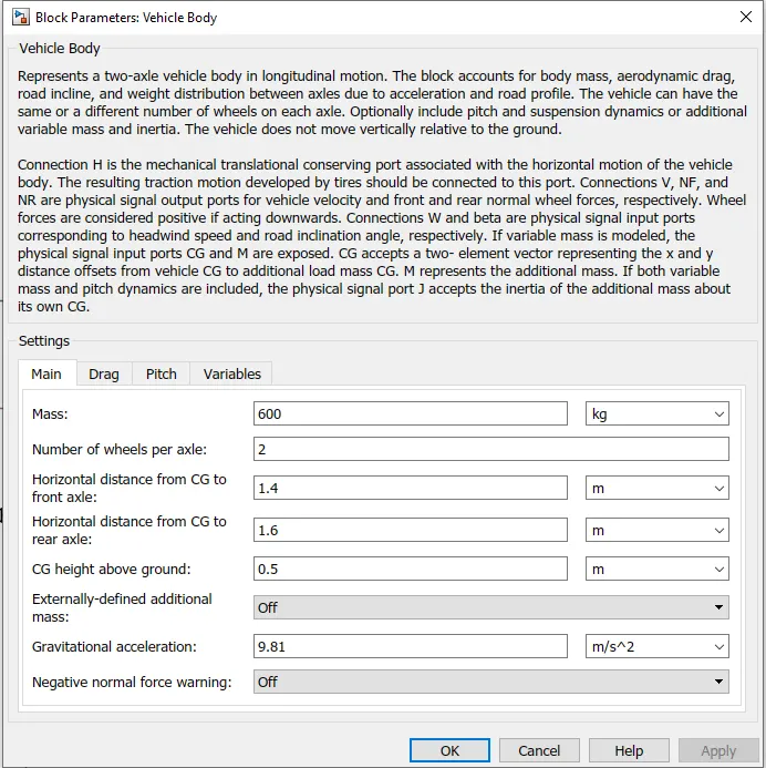
The curb weight of the vehicle is considered as 600 Kgs and the rest all parameters are kept as default.
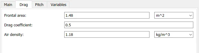
Drag:
Tire (Magic Formula):-
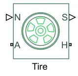
The Tire (Magic Formula) block models a tire with longitudinal behavior given by the Magic Formula, an empirical equation based on four fitting coefficients. The block can model tire dynamics under constant or variable pavement conditions.
The longitudinal direction of the tire is the same as its direction of motion as it rolls on pavement. This block is a structural component based on the Tire-Road Interaction (Magic Formula) block.
PORTS:
S - output port that reports the tire slip
A - It is the mechanical rotational conserving port for the wheel axle
N - input port that applies the normal force acting on the tire
H - It is the mechanical translational conserving port for the wheel hub
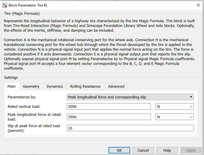
PARAMETERS:
Simple Gear Block:-
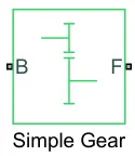
The Simple Gear block represents a gearbox that constrains the connected driveline axes of the base gear, B, and the follower gear, F, to corotate with a fixed ratio that you specify. You choose whether the follower axis rotates in the same or opposite direction as the base axis. If they rotate in the same direction, the angular velocity of the follower, ωF, and the angular velocity of the base, ωB, have the same sign. If they rotate in opposite directions, ωF and ωB have opposite signs.
PARAMETERS:
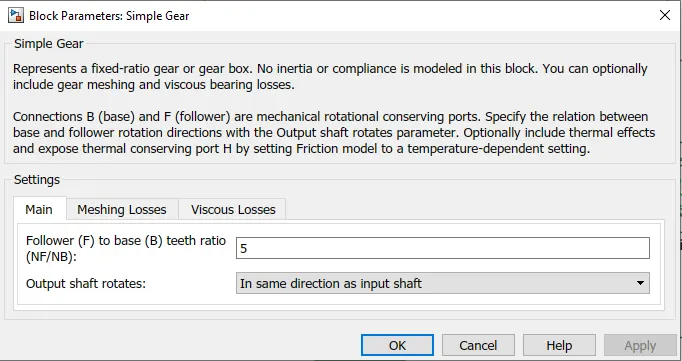
For our modelling we have kept the gear ratio as 5. The more the gear ratio the better the speed along with more traction power. Usually for simulation the gear ratio is kept between 5-10.
Inertia:-
The Inertia block represents an ideal mechanical translational inertia that is described with the following equation:
T=J dω/dt
Battery Subsystem:
The battery subsystem block consists of a Li-ion battery block, a controlled curent source and a voltage measurement block across the battery to measure the battery voltage.
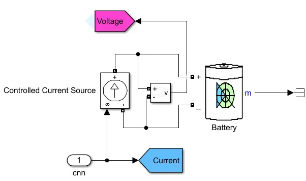
Li-ion Battery Block:-
This battery block implements a generic battery model for most popular battery types such as Lead-acid, Lithium-Ion, Nickel-Cadmium, Nickel-Metal-Hydride. For our model we have selected Li-ion battery type as shown below,
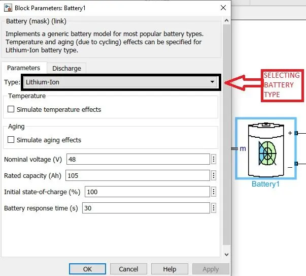
The Li-Ion battery used is of 60 V rated voltage and 630 Ah rated capacity.
Controlled Current Source:-
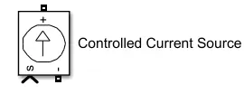
The Controlled Current Source block converts the Simulink input signal into an equivalent current source. The generated current is driven by the input signal of the block. The positive current direction is as shown by the arrow in the block icon.
SOC SUBSYSTEM:
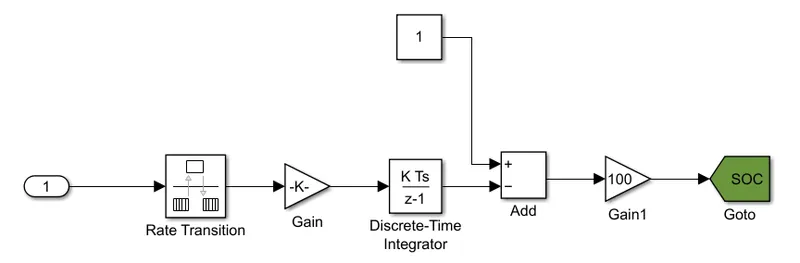
To get the remaining battery capacity after utilization interms of percentage we make use of SOC block. Current from the battery is connected to rate transition block where it transfers data from the output of a block operating at one rate to the input of a block operating at a different rate. This signal is multiplied by a gain value and is fed to the discrete-time integrator block where accumulation of signal takes place. Then this signal is compared with a constant block (considered as 100% full charge) in add block & the output difference value of add block is multiplied by a gain of 100 to get the remaining battery capacity interms of percentage state of charge.
Excel Sheet of all inputs and assumed data:
| Sr No. | Name of the Block | Input Data |
| 1 | Driver Block | |
| 1.1 | Control type | PI |
| 1.2 | Shift Type | None |
| 2 | Battery Subsystem | |
| 2.1 | Battery Type | Li-ion |
| 2.2 | Controlled Current Source | Default inputs |
| 2.3 | Nominal voltage (V) | 60 |
| 2.4 | Rated capacity (Ah) | 630 |
| 2.5 | Initial state-of-charge (%) | 100 |
| 2.6 | Battery response time (s) | 30 |
| 3 | DC Motor Subsystem | |
| 3.1 | Controlled PWM Voltage Block | |
| 3.1.1 | PWM Frequency (Hz) | 1000 |
| 3.1.2 | Simulation Mode | Averaged |
| 3.1.3 | Sample Time (s) | 1.00E-06 |
| 3.1.4 | Output voltage amplitude (V) | 5 |
| 3.2 | DC Motor Block | |
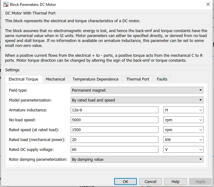
| 3.2.1 | Field type | Permanent Magnet |
| 3.2.2 | Model parameterization | By rated load and speed |
| 3.2.3 | Armature inductance (uH) | 1.20E-05 |
| 3.2.4 | No-load speed (rpm) | 5000 |
| 3.2.5 | Rated speed (at rated load) (rpm) | 1500 |
| 3.2.6 | Rated load (mechanical power) (kW) | 20 |
| 3.2.7 | Rated DC supply voltage (V) | 60 |
| 3.2.8 | Rotor damping parameterization | By damping value |
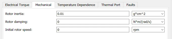
| 3.2.9 | Rotor inertia (g*cm^2) | 0.01 |
| 3.2.10 | Rotor damping (N*m/(rad/s)) | 0 |
| 3.2.11 | Initial rotor speed | 0 |
| 4 | Vehicle Dynamics | |
| 4.1 | Gearbox | |
| 4.1.1 | Follower (F) to base (B) teeth ratio (NF/NB) | 5 |
| 4.1.2 | Output shaft rotates | In same direction as input shaft |
| 4.2 | Tire (Magic Formula) (Same for all three tires) | |
| 4.2.1 | Main | Default values |
| 4.2.2 | Geometry | |
| 4.2.3 | Rolling radius (m) | 0.3 |
| 4.3 | Vehicle Body Block | |
| 4.3.1 | Mass (kg) | 600 |
| 4.3.2 | Number of wheels per axle | 2 |
| 4.3.3 | Horizontal distance from CG to front axle (m) | 1.4 |
| 4.3.4 | Horizontal distance from CG to rear axle (m) | 1.6 |
| 4.3.5 | CG height above ground (m) | 0.5 |
| 4.3.6 | Externally-defined additional mass | Off |
| 4.3.7 | Gravitational acceleration (m/s^2) | 9.81 |
| 4.3.8 | Negative normal force warning | Off |
| 4.3.9 | Drag | |
| 4.3.10 | Frontal area (m^2) | 1.48 |
| 4.3.11 | Drag coefficient | 0.5 |
| 4.3.12 | Air density (kg/m^3) | 1.18 |
RESULT
1. FTP75
Speed
The Electric Rickshaw model efficiently follows the input drive cycle.
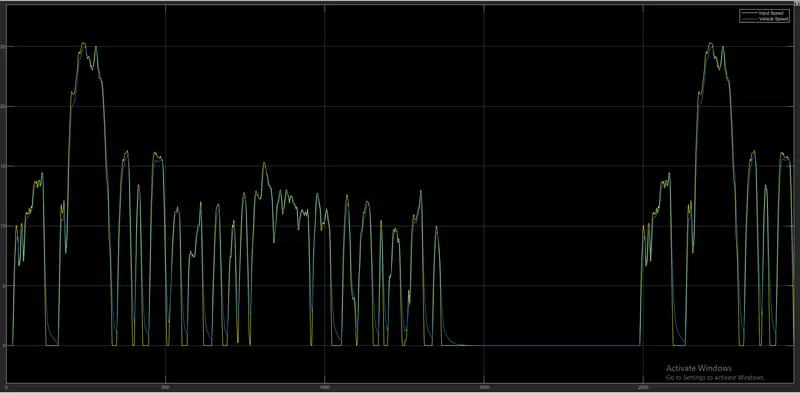
As we can see we got the velocity profile almost completely following the drive cycle data with the maximum speed reaching up to 25km/hr.
Distance Covered
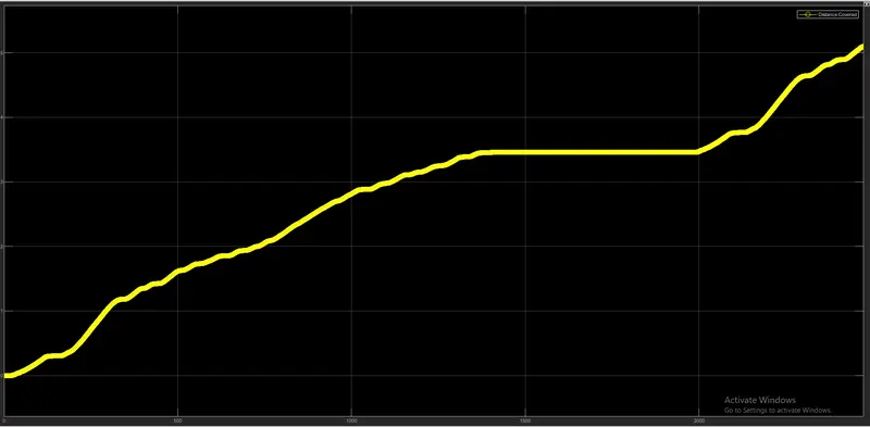
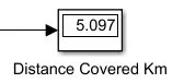
From the output plot of distance covered we can see that by running the Vehicle with F1P75 Drive cycle for 2474 see the distance traveled is 5.097 km. The gear ratio in the simple gearbox is kept at 5.
SOC, Current & Energy Consumed
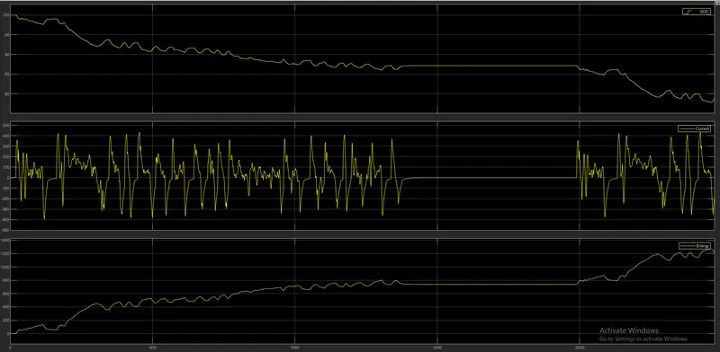
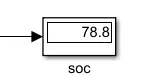
The state of charge for the battery drop to 78.8% of its 100% value for the complete drive cycle. It covered a distance of 5.097 km by utilising 21.2% charge from the battery.
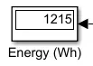
The required by the vehicle to travel a distance of 5.097 km is 1.215 kWh.
AS per the drive current follows positive and negative profile. Positive being current drawn from the battery and negative being current drawn inside the battery(regeneration). That is where the SOC increases.
Motor & Controller Temperature
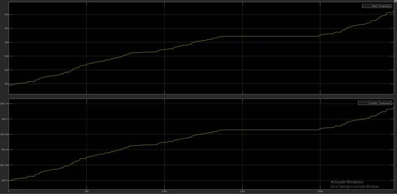
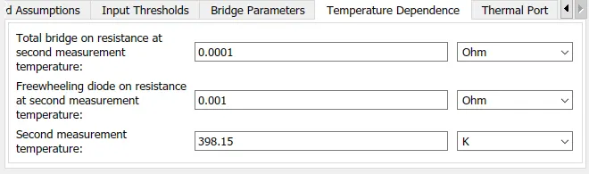
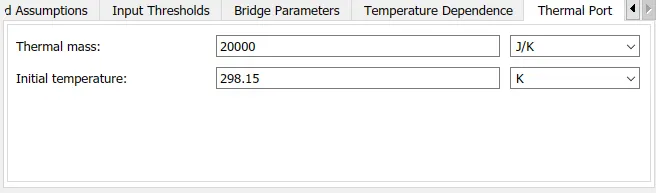
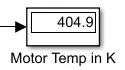
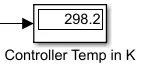
The temperature of the Motor is increased to 404.9K whereas the temperature of the Controller is 298.2K with 20000 as the thermal mass given both to the motor and the H - bridge.
2. WOT (60 seconds)
Speed
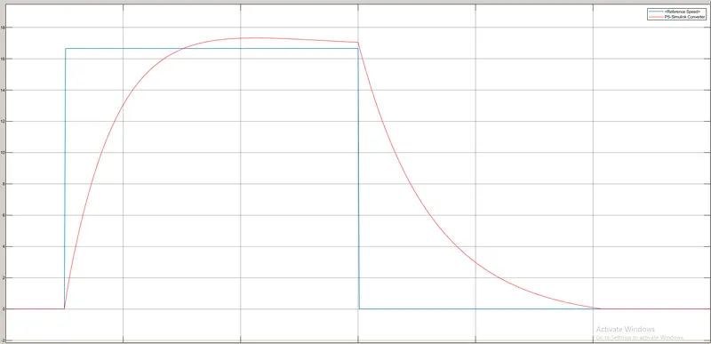
It is clear from the plot that the vehicle speed follows the input speed of drive cycle. Due to inertial effects and instantaneous velocity variation, the actual velocity curve (orange curve) of model varies from that of WOT condition velocity curve (blue curve).
Distance Covered
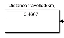
By running the vehicle with WOT (60 seconds) drive cycle the total distance covered is 0.4667km.
SOC & Current
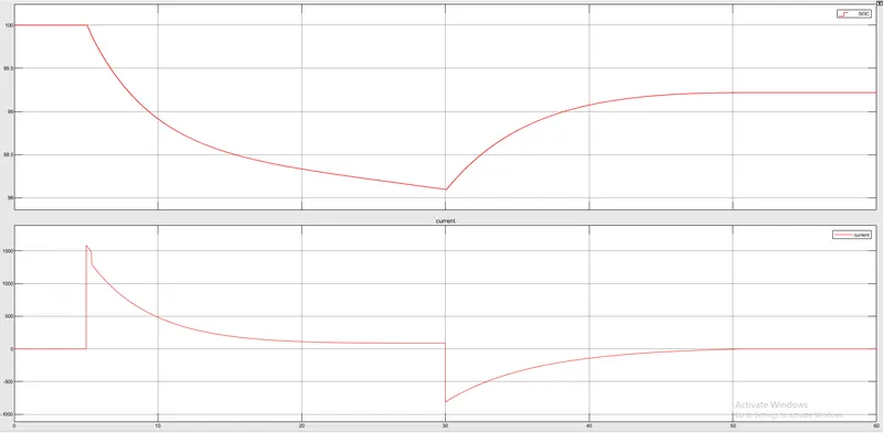
To cover a distance of 0.4667km the vehicle consumed 0.78% of of total charge from the battery. The State of Charge of the battery is 99.22%. It can be seen that whenever there is an deceleration the battery gets charged due to regenerative braking effect.
Motor & Controller Temperature
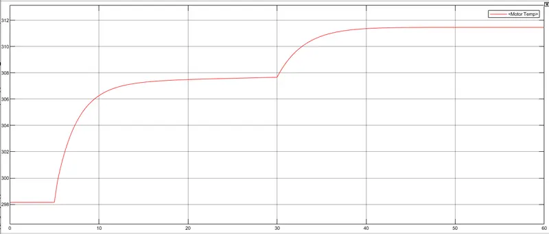
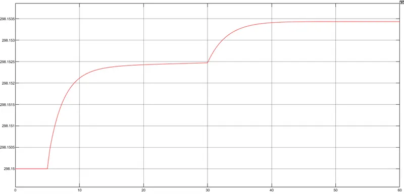
Due to sudden acceleration in WOT drive cycle, the current drawn from the battery will also be very high. This causes the motor temperature rise
upto 311.5K and the controller temperature is nearly 298.15K.
3.Userdefined Drive Cycle
Speed
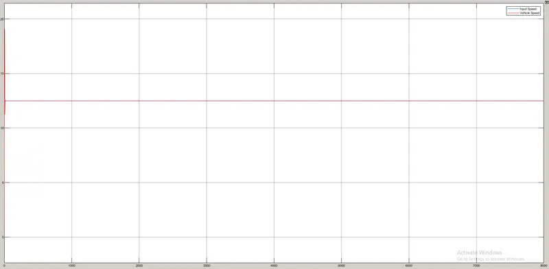
For this user defined drive cycle we are getting the velocity profile almost completely following the drive cycle data with the maximum speed reaching up to 12.5km/hr.
Distance Covered
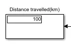
The distance covered by the vehicle at constant speed 45kmph is 100km which matches with the actul distance covered by drive cycle.
SOC & Current
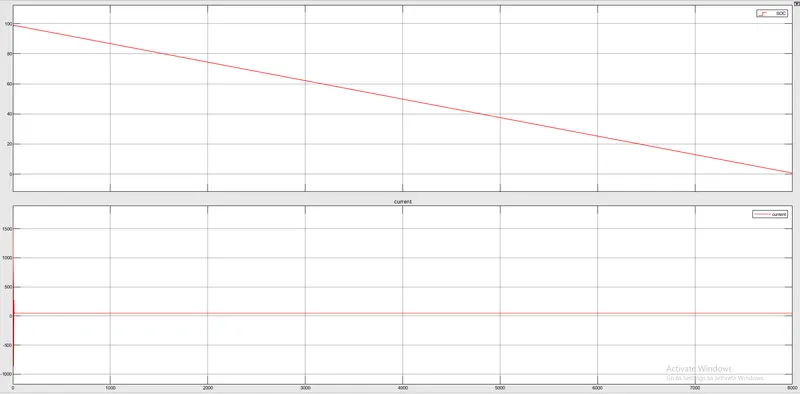
The SOC of the battery is found to be only 0.64% of total capacity. This is because to cover the distance of 100km constant speed of @45kmph, the vehicle needs much higher energy from the battery. Here the large current of 48.7A is drawn from the battery throghout the drive cycle. Thus it takes around 99.35% of full charge to cover the distance of 100km.
Motor & Controller Temperature
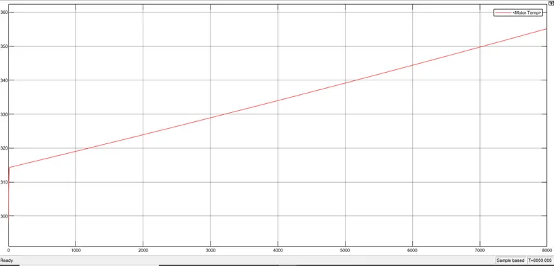
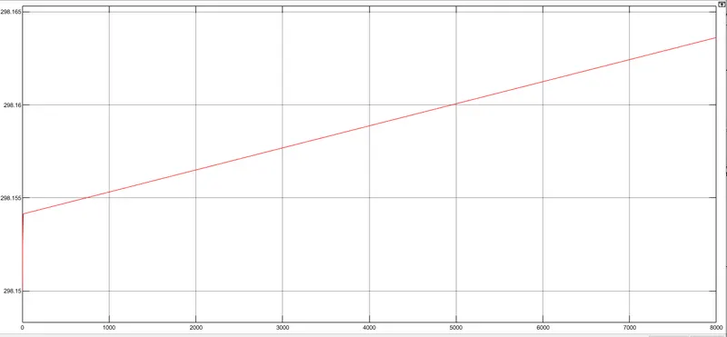
Due to high current drawn from the battery the motor temperature rised to 355K and the controller temperature was 298.16K.
CONCLUSION:
- In the speed comparison plots for all the drive cycles which are discussed in this study, the feedback/actual speed plot and the reference speed plot overlap each other almost completely but there are some regions where both speeds are different. It is when vehicle is decelerating. The reference speed graph falls sharply but actual/feedback speed doesn't. This is because of the inertia of the vehicle body. As the inertia of vehicle body is higher, it takes a longer duration for it to decelerate. That is why the overlapping is not 100%.
- In this study, Electric Rickshaw and its components have been simulated in order to investigate the energy flow, performance and efficiency. Good results for Battery Voltage, Current, and Power were shown by using MATLAB-Simulink.
- From the simulation we can say that the Electric Rickshaws are much more efficient compared to the traditional Auto-rickshaw as they are non-polluting and the power loss is comparatively less.