Final Project: Design of an Electric Vehicle

AIM

To create a MATLAB model of electric car which uses a battery and a DC motor using Power train block set.

OBJECTIVE

To model an electric car in MATLAB using Power train block set and prepare a report including following:

1. System level configurations
2. Model parameters
3. Results
4. Conclusion

DESIGN CALCULATIONS

To model the EV, we have to calculate certain parameters like, Power, Energy, Range, Motor Rating, Battery Capacity etc. For Vehicle dimension data, let’s refer TATA NEXON EV Spec. which is given below.

TATA NEXON EV – Specifications

Power	95kW
Length (mm)	3993
Width (mm)	1811
Height (mm)	1606
Tire Dimension	664.4mm
Kerb Weight (Kg)	1400
Battery Capacity	30.2kWh
Motor Ratings (3phase PMSM)	97.46kW, 245Nm
Range	312km

Table 1: TATA Nexon Specifications

In order to find the motor ratings, Battery capacity, Maximum power, Torque and Energy required by the vehicle, we have to create a model first for the design of Electric vehicle.

To calculate the parameters of the vehicle, let’s first choose the drive cycle.

Drive cycle

The WLTP procedure (world harmonized light-duty vehicles test procedure) is a harmonized standard for determining the levels of pollutants, CO₂ emissions and fuel consumption of traditional and hybrid cars, as well as the range of fully electric vehicles.

The WLTP procedure relies on the new driving cycles (WLTC – Worldwide harmonized Light-duty vehicles Test Cycles) to measure the mean fuel consumption, the CO₂ emissions as well as the emissions of pollutants by passenger cars and light commercial vehicles.

The test procedure WLTP (Worldwide harmonized Light vehicles Test Procedure) contains several driving cycles:

• Class 1 – low power vehicles with PW_r <= 22
• Class 2 – vehicles with 22 < PW_r <= 34
• Class 3 – high-power vehicles with PW_r > 34

Where PW_r [kW/Tonne] is the power-to-weight ratio, defined as the ratio between the rated engine power and kerb weight.

PWr=Pmax/mv

Since we are modeling TATA Nexon EV, Let’s take parameters from Table 1.

Pmax =95kW , Kerb Weight = 1.4 Tonnes

PWr= 95/1.4 = 67.85

Since the vehicle’s PW_r is bigger than 34, we are going to use the WLTC Class 3 driving cycle to calculate the energy consumption.

WLTC Class 3

The WLTP is divided into 4 different sub-parts, each one with a different maximum speed:

• Low, up to 56.5 km/h
• Medium, up to 76.6 km/h
• High, up to 97.4 km/h
• Extra-high, up to 131.3 km/h.

These driving phases simulate urban, suburban, rural and highway scenarios respectively, with an equal division between urban and non-urban paths (52% and 48%).

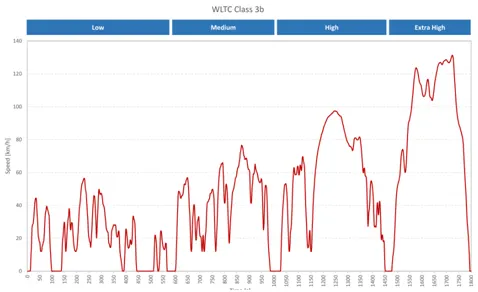
Figure 1: WLTC Class 3b Driving Cycle

Force Calculation

The forces acting on the vehicle are as follows.

Rolling Resistance = m*g*Cr*cos(alpha) = 1000*9.81*0.02*cos(1)

Aerodynamic drag = 0.5*Cd *Af*Ad*V^2 = 0.5* 0.33*2.34*1.25*V^2

Grade Resistance = m*g*sin(beta) = 1000*9.81*sin(10)

Acceleration resistance = m*a = 1000*(Velocity difference)

Total force = Sum of all the above forces.

Power = Total Force * Velocity

Torque = Power * Wheel radius

Energy = 1/s (Power)

The above calculations can be modeled in Simulink as shown below.

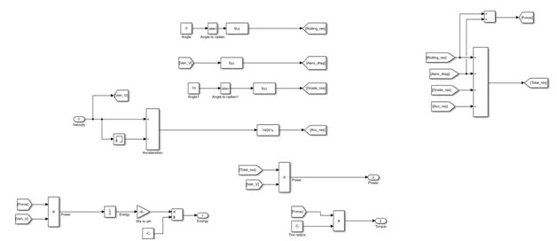
Figure 2: Modeling Forces and calculating Torque, Enegy and Power

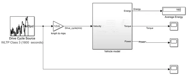
Figure 3: Vehicle Model in Simulink

By dividing the last calculated value of the total energy to the total length of the WLTC drive cycle (23.266 km), we get the average energy consumption of the vehicle, 160 Wh/km.

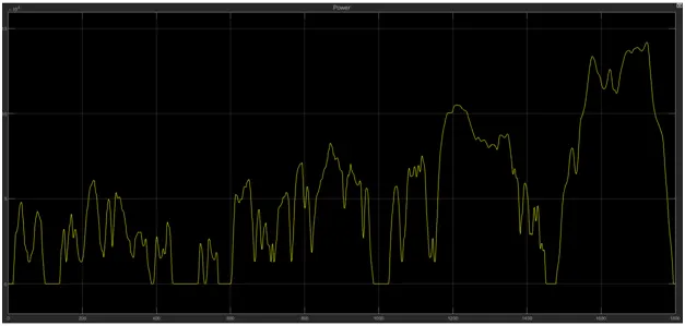
Figure 4: Power Curve of Vehicle

The above plot gives the power required by the vehicle at different speeds of drive cycle. From the plot we can understand that in order to achieve maximum speed of 131km/hr, the motor should be rated with 140kW. But due to size and cost constraint we cannot choose the high rated motor. We should select in such a manner that the motor operated at maximum efficiency during average speed.

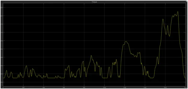
Figure 5: Torque Curve

From the above plot, we can understand that the maximum required torque is 222Nm.

Motor Capacity Selection

Form the Torque and power plots we can select the motor required for our Electric Car. As we are modeling TATA Nexon, we can choose BLDC motor with 95.8kW, 279Nm.

The Parameters of Motor from figure 6 can be summarized in the table below.

Rated Power	95.8 kW
Rated Torque	279Nm
Rated voltage	460V
No load Speed	3280rpm
Rated Speed	4000rpm
Armature Inductance	2mH

Table 2: Motor Ratings

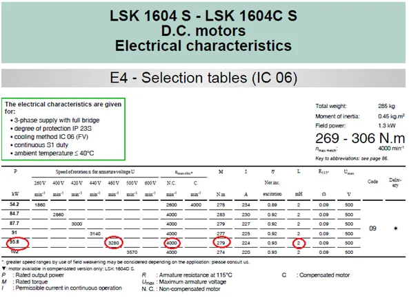
Figure 6: Motor Rating

Battery Capacity Calculations [2],[3]

We have calculated the average energy consumption for propulsion E_p as being 160 Wh/km on WLTC drive cycle. On top of the energy needed for propulsion, the high voltage battery must supply the energy for the vehicle’s auxiliary devices E_aux [Wh/km], like: 12 V electrical system, heating, cooling, etc. Also, we have to consider the efficiency of the powertrain η_p during the conversion from electrical energy to mechanical energy.

Eavg=(Ep+Eaux)/ η_p                                                                                                                                                (1)

The prolonged electrical loads (headlights, multimedia, etc.) and intermittent loads (heater, brake lights, wipers, etc.) use on average 430 W of electrical power. The duration of the WLTC cycle is 1800 s (0.5 h), which gives an energy of 215 Wh for the auxiliary loads. If we divide it to the length of the WLTC driving cycle (23.266 km), we get an average energy consumption for the auxiliary loads E_aux of 9.241 Wh/km.

Even if Wh/km is not really energy but factorised energy, since it’s dived per unit of distance (km), for simplicity, we are going to refer to it as average energy.

The direct current (DC) supplied by the battery is converted into alternated current (AC) by the inverter. This conversion is taking place with an associated loss. Also, the electric motor and driveline have some losses which we need to consider. For this exercise we are going to use an average efficiency η_p of 0.9 from the battery to the wheel.

Replacing the values in (1) gives the average energy consumption:

Eavg=(160+9.241)/0.9=188.045 Wh/km

The battery pack will be designed for an average energy consumption of 188.045 Wh/km.

The required battery pack total energy E_bp [Wh] is calculated as the product between the average energy consumption E_avg [Wh/km] and vehicle range D_v [km]. For this example we’ll design the high voltage battery pack for a vehicle range of 250 km.

Ebp=Eavg * Dv=188.045 * 250 = 47,011.25 Wh=47.011 kWh                                                       (2)

The following calculations are going to be performed for each cell type. For this example we are going to consider that the battery pack is made up only from several strings connected in parallel.

The number of battery cells connected in series (N_cs) in a string is calculated by dividing the nominal battery pack voltage U_bp [V] to the voltage of each battery cell U_bc [V]. The number of strings must be an integer. Therefore, the result of the calculation is rounded to the higher integer.

Ncs = Ubp * Ubc = 460 / 3.6 = 128                                                                                                     (3)

The energy content of a string E_bs [Wh] is equal with the product between the number of battery cells connected in series N_cs and the energy of a battery cell E_bc [Wh].

Ebs = Ncs * Ebc = 128 * 11.52 = 1474.56Wh                                                                                    (4)

The total number of strings of the battery pack (N_sb) is calculated by dividing the battery pack total energy E_bp [Wh] to the energy content of a string E_bs [Wh]. The number of strings must be an integer. Therefore, the result of the calculation is rounded to the higher integer.

Nsb=Ebp / Ebs = 47011.25 / 1474.56 = 32                                                                                        (5)

We can now recalculate the battery pack total energy E_bp [Wh] as the product between number of strings N_sb and the energy content of each string E_bs [Wh].

Ebp=Nsb*Ebs  = 32*1474.56 = 47185.92 Wh                                                                                   (6)

The battery pack capacity C_bp [Ah] is calculated as the product between the number of strings N_sb and the capacity of the battery cell C_bc [Ah].

Cbp = Nsb*Cbc = 32 * 3.2 = 102.4 Ah                                                                                                 (7)    

The total number of cells of the battery pack (N_cb) is calculated as the product between the number of strings N_sb and the number of cells in a string N_cs.

Ncb = Nsb*Ncs = 32*128 = 4096                                                                                                       (8)   

The Battery Parameters can be summarized in the following table.

Vehicle Range	250 km
Average Energy Consumption	188.045 Wh/km
Nominal voltage of single cell	3.6V
Capacity of single cell	3.2Ah
Energy of a single cell	11.52Wh
No. of cells in a string	128
No. of Strings	32
Total no.of cells	4096
Nominal Battery Voltage	460V
Energy of Battery pack	47.19kWh
Power of battery pack	47.10kW
Battery Current	102.40A
Capacity of Battery pack	102.40Ah

Table 3: Battery Ratings

SIMULINK MODELLING OF COMPLETE ELECTRIC VEHICLE

The Complete model of Electric vehicle in Simulink is as shown below in figure 7.

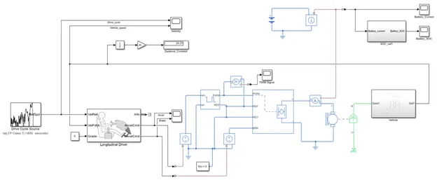
Figure 7: Simulink Model of Electric Vehicle

The modelling of each parameters are explained below.

1. Longitudinal Driver

The Library to access Longitudinal Driver is given below.

Library: Powertrain Blockset / Vehicle Scenario Builder

Vehicle Dynamics Blockset / Vehicle Scenarios / Driver

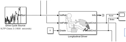
Figure 8: Longitudinal Driver

For velocity Reference (VelRef), we can connect the drive cycle WLTP Class 3 which we have used for design calculations. Velocity feedback is the actual vehicle velocity. Grade is the inclination of road, which we have given 0. According to the error between actual and reference velocity, Acceleration and Deceleration signals are generated.

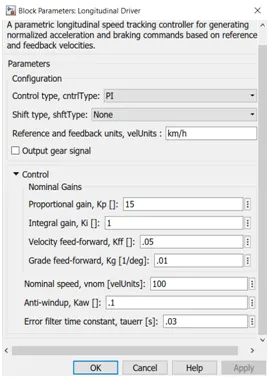
Figure 9: Longitudinal Driver Parameters

The control parameters are kept same as shown above.

2. Pulse-width modulated voltage source

The Library to access PWM source is given below.

Library:           

Simscape / Electrical / Integrated Circuits

This block will generate PWM signals according to the reference signal given to it.

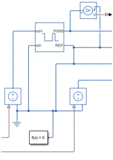
Figure 10: PWM Source

The PWM frequency is given as 4000Hz as shown below. The Input is coming from Longitudinal driver Accel and Decel ports, and it will vary from 0 to1. Those signals are converted to equivalent voltages using controlled voltage source block as shown in figure 10.

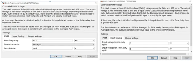
Figure 11: Controlled PWM Voltage Parameters

The Output voltage of the PWM is set as 5V.

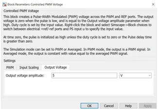
Figure 12: PWM Output Voltage

3. H-Bridge

The library to access H-Bridge is given below.

Library:           

Simscape / Electrical / Semiconductors & Converters / Converters

The H-bridge can control the DC motor according to the PWM signals given to it. It can take supply from external power supply  or internal one. Here I’ve choose internal power supply.

The H-Bridge block represents an H-bridge motor driver. The block has the following two Simulation mode options:

PWM — The H-Bridge block output is a controlled voltage that depends on the input signal at the PWM port.

Averaged — This mode has two Load current characteristics options:

Smoothed

Unsmoothed or discontinuous

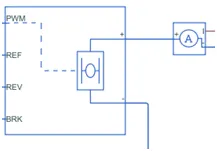
Figure 13: H-Bridge

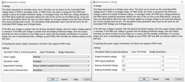
Figure 14: H-Bridge Parameters

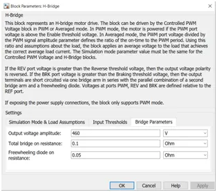
Figure 15: H-Bridge Output Voltage

The PWM signal amplitude is same as that of given in PWM Source. The output voltage is same for motor rated voltage and battery.

4. DC Motor

The library to access DC Motor is shown below.

Library: Simscape / Electrical / Electromechanical / Brushed Motors

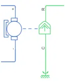
Figure 16: DC Motor

When the Model parameterization parameter is set to By rated power, rated speed & no-load speed, the block uses the rated speed and power to calculate the rated torque. The block uses the rated torque and no-load speed values in the preceding equation to determine values for R and kt.

The resistor R corresponds to the resistance you specify in the Armature resistance parameter. The inductor L corresponds to the inductance you specify in the Armature inductance parameter. The permanent magnets in the motor induce the following back emf vb in the armature:

Vb = kv*w

where kv is the Back-emf constant and w is the angular velocity. The motor produces the following torque, which is proportional to the motor current i:

Te = kt*i

where kt is the Torque constant.

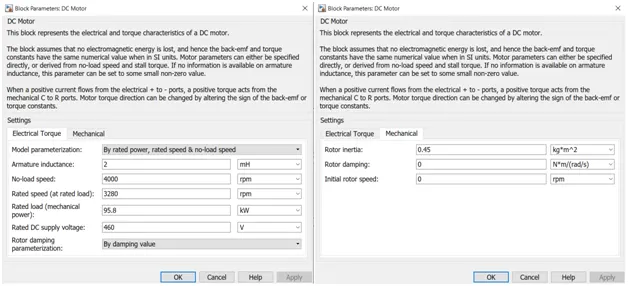
Figure 17: DC Motor Parameters

The motor parameters are given based on the values given in Table 2.

5. Battery

The battery model can be accessed from the following library.

Library: Simscape / Electrical / Sources

The Battery block represents a simple battery model. The block has four modeling variants, accessible by right-clicking the block in your block diagram and then selecting the appropriate option from the context menu, under Simscape > Block choices:

Uninstrumented | No thermal port — Basic model that does not output battery charge level or simulate thermal effects. This modeling variant is the default.

Uninstrumented | Show thermal port — Model with exposed thermal port. This model does not measure internal charge level of the battery.

Instrumented | No thermal port — Model with exposed charge output port. This model does not simulate thermal effects.

Instrumented | Show thermal port — Model that lets you measure internal charge level of the battery and simulate thermal effects. Both the thermal port and the charge output port are exposed.

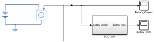
Figure 18: Battery Model

Here I’ve used Unintrumented | No thermal port model. The battery fade, dynamics and self discharging has been disabled.

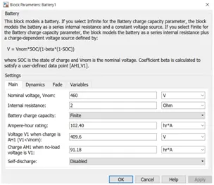
Figure 19: Battery Parameters

The nominal voltage of the battery is set as 460V which is same as that of motor rated voltage. The battery rating is given as per Table 3 data.

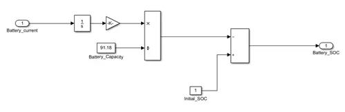
Figure 20: Battery SOC Estimation

In order to determine State Of Charge of the battery, we can use coulomb counting method.

In this method we are subtracting the charge taken from the battery to the initial SOC.

SOC(t) = SOC(t-1)  – (I*t) / AH

The above equation can be modelled in simulink as figure 20.

6. Vehicle Model

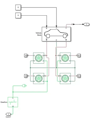
Figure 21: Vehicle Model

The vehicle model subsystem consists of the following blocks.

1. Vehicle body
2. Tire
3. Gear

• Vehicle Body

Two-axle vehicle with longitudinal dynamics and motion and adjustable mass, geometry, and drag properties.

Library: Simscape / Driveline / Tires & Vehicles

The Vehicle Body block represents a two-axle vehicle body in longitudinal motion. The vehicle can have the same or a different number of wheels on each axle. The vehicle wheels are assumed identical in size. The vehicle can also have a center of gravity (CG) that is at or below the plane of travel.

The block accounts for body mass, aerodynamic drag, road incline, and weight distribution between axles due to acceleration and road profile. Optionally include pitch and suspension dynamics. The vehicle does not move vertically relative to the ground.

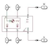
Figure 22: Vehicle body

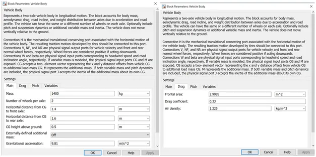
Figure 23: Block Parameters of Vehicle body

The values of Mass, Frontal area, drag coefficient values given in the vehicle body are from table 1, TATA NEXON specifications.

• Tire

Tire with longitudinal behaviour given by Magic Formula coefficients.

Library:           

Simscape / Driveline / Tires & Vehicles

The Tire (Magic Formula) block models a tire with longitudinal behaviour given by the Magic Formula, an empirical equation based on four fitting coefficients. The block can model tire dynamics under constant or variable pavement conditions.

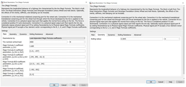
Figure 24: Tire Parameters

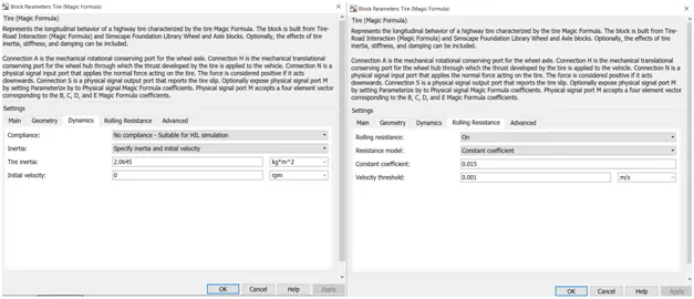
Figure 24b: Tire Parameters

I’ve chosen Load dependent magic formula coefficients. The tire inertia and rolling radius values have been taken from Table 1 Tata NEXON Specifications.

• Gear

Simple gear of base and follower wheels with adjustable gear ratio, friction losses, and triggered faults. It can be accessed from the following libaray.

Library: Simscape / Driveline / Gears

The Simple Gear block represents a gearbox that constrains the connected driveline axes of the base gear, B, and the follower gear, F, to co rotate with a fixed ratio that we specify. We can choose whether the follower axis rotates in the same or opposite direction as the base axis. If they rotate in the same direction, the angular velocity of the follower, ωF, and the angular velocity of the base, ωB have the same sign. If they rotate in opposite directions, ωF and ωB have opposite signs.

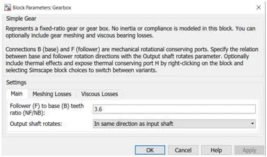
Figure 25: Gear Parameters

RESULT ANALYSIS

The distance covered by the vehicle can be found from the block given below. By integrating the vehicle velocity we will get the distance covered. The velocity is in km/hr and the integration time is in seconds. So we have to multiply the displacement by a 1/3600 to convert it in to hours. Then the answer we are getting will be distance in km.

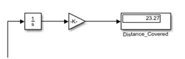
Figure 26: Distance Covered by the Vehicle

The distance covered by the vehicle in WLTP Class 3 drive cycle is 23.27km.

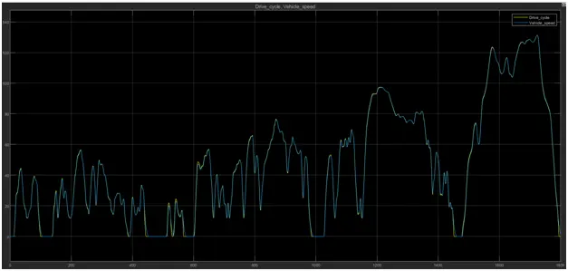
Figure 27: Drive cycle and Vehicle speed plot

The above figure shows the drive cycle speed and vehicle speed plot. We can see that vehicle follows drive cycle in all regions. Slight variations in the curve are in the regions of sudden braking. This may be due to the inertia of the tires.

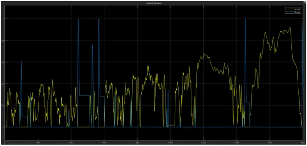
Figure 28: Acceleration and Deceleration plot

The acceleration and brake signals developed by longitudinal driver is shown above.

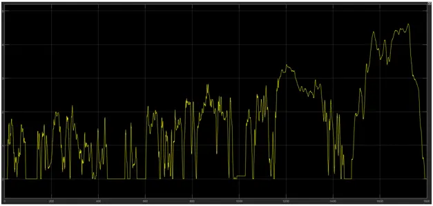
Figure 29: PWM Signal to the H-Bridge

The PWM signal generated according to control signals given is shown above. The magnitude of the signal varies with required speed. During maximum speed, the magnitude is maximum and during braking, magnitude is zero.

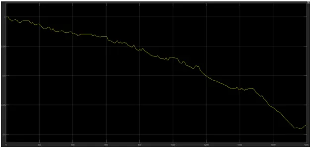
Figure 30: Battery SOC plot

The State Of Charge plot of the battery is given above. From the plot we can understand that during acceleration, battery is discharging and during braking battery is charging due to regenerative braking enabled in H-bridge. By the end of trip, the SOC has reached 82%.

CONCLUSION

MATLAB model of electric car has been created and driver, vehicle and motor parameters were analysed. The design consideration for electric has been analysed with equation based simulink model. Motor rating and battery rating have chosen from datasheet based on calculations in the model. We could also analyse the vehicle velocity and SOC of battery plot.