Design of an Electric Vehicle

Design of an Electric Vehicle

Aim:

Creating a Simulink model of an Electric Car using a battery and a DC motor

Theory:

The three main components of EV vehicles are;

1. Battery

2. Motor

3. Controls

Motors and Controls both account for the DC Drive.

For the EV Drivetrain, I have used Brushless DC Motor, Simple Voltage Source, and PWM signal.

EV batteries undergo cycles of 'discharge' that occur when driving and 'charge' when the car's plugged in. Repeating this process over time affects the amount of charge the battery can hold. This decreases the range and time needed between each journey to charge.

Battery and electric motor working together is surprisingly simple – the battery connects to one or more electric motors, which drive the wheels. When you press the accelerator the car instantly feeds power to the motor, which gradually consumes the energy stored in the batteries. Electric motors also work as generators, so when you take your foot off the throttle the car begins to slow down by converting its forward motion back into electricity – this happens more strongly if you hit the brakes. This regenerative braking recovers energy that would otherwise be lost, storing it in the battery again and so improving the car's range.

Procedure:

At first, we will design the body of the vehicle. The body will compromise of four wheels. The wheels are getting the power from the motor but only after getting through the transmission, which in this case in Simple Gear.

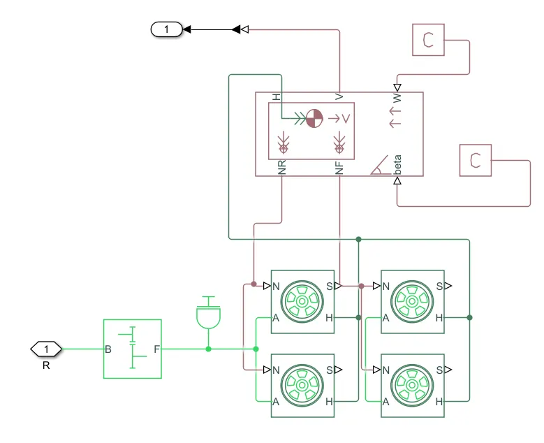
Fig: Vehicle Body

We will create a subsystem of these blocks. Then, the motor will be made using the Brushless DC Motor.

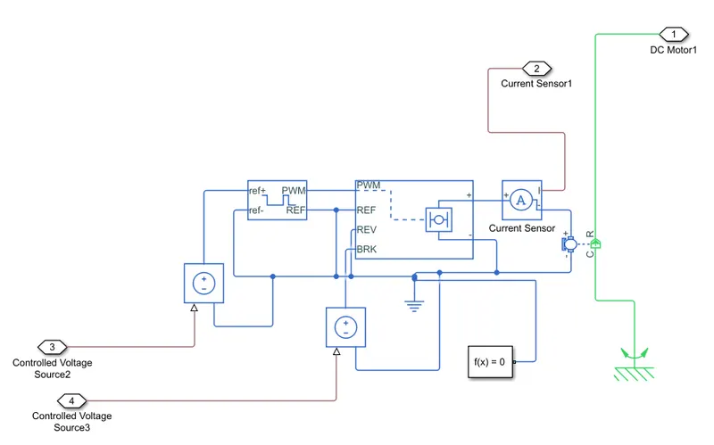
Fig: DC Drive

We will make use of the H-Bridge Rectifier to convert AC current to DC current. For the Duty Cycle, a PWM block is used. All of the negative ends are connected to the electrical reference. Again this will be created a separate subsystem.

Once this is done, the power source is created.

The Simple voltage source is used for this purpose. The Negative end goes to electrical reference, whereas the positive end goes to the motor to provide the drive. A control current source is used. This is created a separate subsystem.

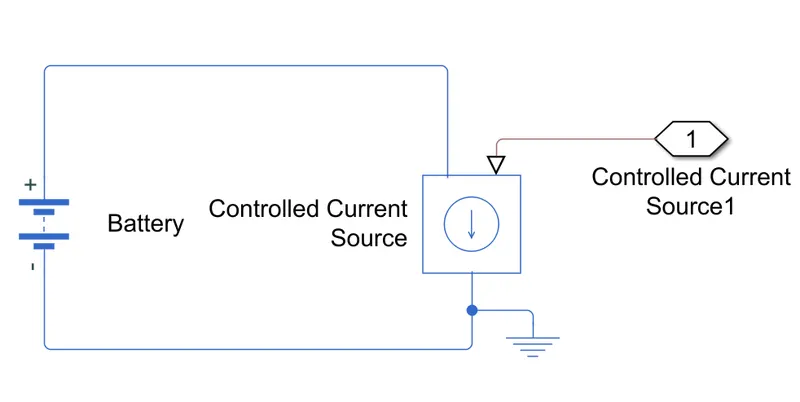
Fig: Battery

Once this is done, we will configure them. The following is the configuration of the Battery, DC drive, and Vehicle Body. Battery and Motor plays a pivotal role, as a result, they need to be configured properly.

First, for the battery, the Nominal Voltage is set at 300V. Internal resistance is set at 2 Ohm. The battery is 25 Ah capacity.

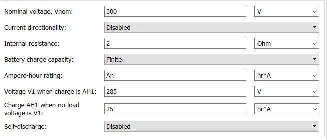
Fig: Configuration of Battery

Secondly, the motor is configured. The Voltage here needs to be higher than the voltage by the battery. Here it is set at 330 V. The total bridge on-resistance is set at 0.1 Ohm, whereas freewheeling diode resistance is taken as 0.05 Ohm.

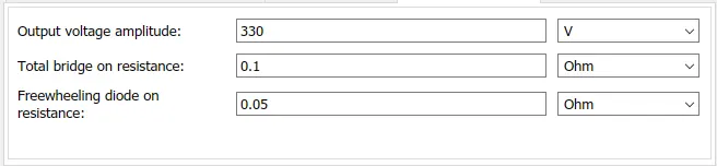
Fig: Configuration of Brushless DC Motor

Thirdly, the PWM signal is configured. Here the frequency is set at 4000 Hertz whereas the Simulation mode is set at Average.

Fig: Configuration of PWM Signal

Lastly, for Vehicle Body, the total mass is considered as 800 kg. Rest we will configure with an educated guess. I have kept the default values. The number of the wheel per axle is taken as 2.

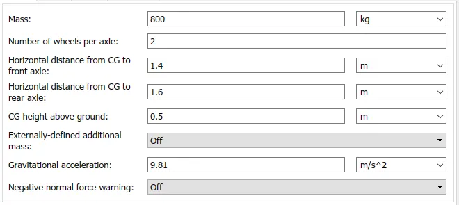
Fig: Configuration of Vehicle Body

To provide the input to it, we will provide the Longitudinal Driver. The Vehicle feedback is provided by the output of distance covered. Acceleration and deceleration are provided to the motor. The grade is assumed as 0.

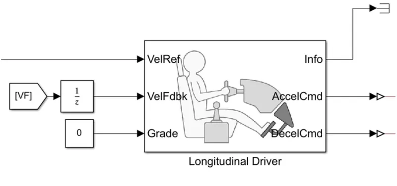
Fig: Longitudinal Driver

To provide traction, we need a particular input from the user. The input can is the power required for a particular speed. That is at every time interval we need the speed required at a particular load.

For this model, I have selected FTP75 Drive Cycle. Using Signal Builder block the input can be provided. The Slider gain is another method of providing the input. The electric powertrain can also be given using the excel sheet data of time v/s speed.

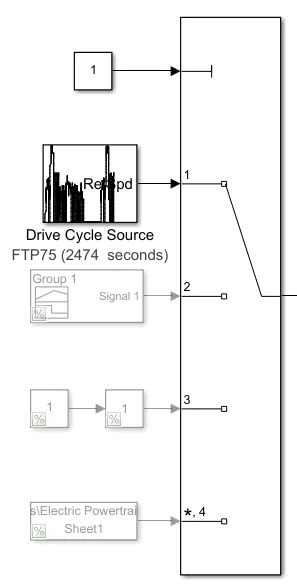
Fig: List of Drive Cycle provided

The State of Charge is calculated with the current drawn from the battery. The following represents the conversion of the current into a state of charge. The difference between this with 1 will give the Actual State of Charge.

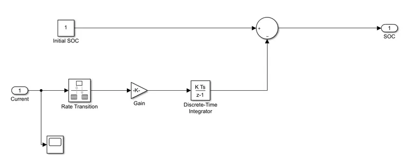
Fig: SOC Calculator

The output from the vehicle body is integrated at every time interval and it is divided by 1000 to convert into a kilometer.

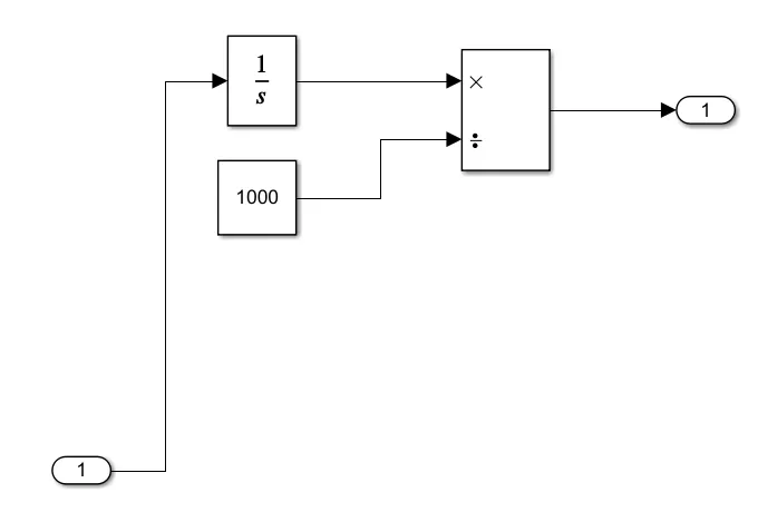
Fig: Distance covered Calculator

Both of these are put into a subsystem. The subsystem to calculate SOC and Distance covered.

I have used dashboard output for better visualization. The Display block is used for showcasing distance. The Speed and SOC are depicted by Full and Half Gauge Block. The current drawn is shown by the vertical gauge.

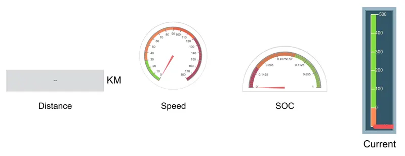
Fig: Dashboard

The final model is as follow;

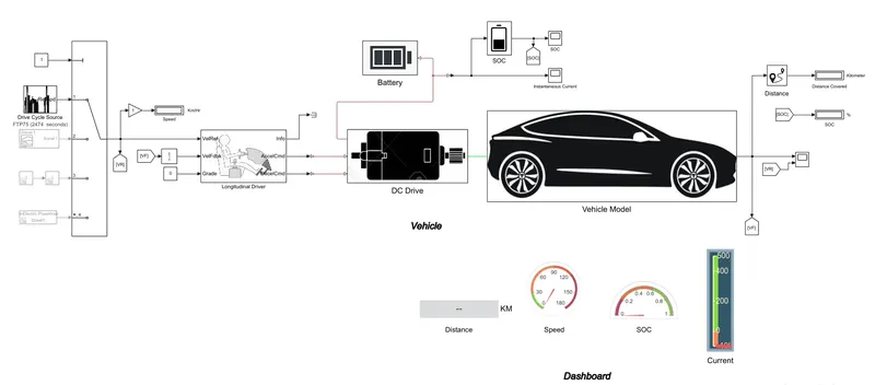
Fig: Final Model of an Electric Vehicle

For better visualization, the subsystem is masked with the image icon.

Result:

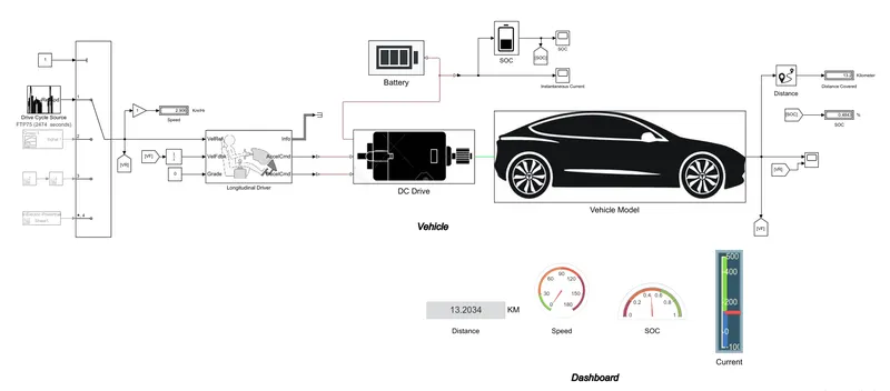
Fig: Final Model of the Electric Vehicle with FTP75 Drive Cycle Result

The following is the Simulation of an Electric Vehicle

The following is the State of Charge while driving. When the vehicle applies the brakes the SOC is increasing marginally. Whereas, it decreases during the drive.

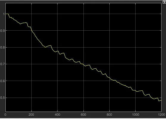
Fig: State of Charge

The following is the output of Drive coming from Multiport Switch and the output of Vehicle Model. They are almost the same.

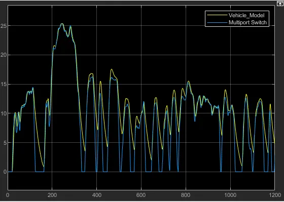
Fig: Input of Multiport Switch and Vehicle Model

The following is the result of the current drawn from the battery during the drive. It can be seen that it goes negative, it is because during the event of brake the battery gets charged due to regenerative braking.

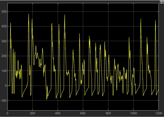
Fig: Current drawn from the battery

Conclusion:

Created a MATLAB model of an Electric Car using a battery and a DC motor. The car covered nearly 13.2 km with FTP75 drive cycle in 1200 seconds. The SOC was almost halved during the drive.