Final Project: Design of an Electric Vehicle

Aim: Create a MATLAB model of an electric car which uses a battery and a DC motor.

Objective:

1. System level configuration.
2. Model parameters.
3. Results.
4. Conclusion.

Electric Car:

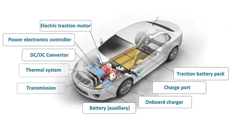
All-electric vehicles (EVs), also referred to as battery electric vehicles, have an electric motor instead of an internal combustion engine. The vehicle uses a large traction battery pack to power the electric motor and must be plugged into a wall outlet or charging equipment, also called electric vehicle supply equipment (EVSE). Because it runs on electricity, the vehicle emits no exhaust from a tailpipe and does not contain the typical liquid fuel components.

Traction battery pack:

Stores electricity for use by the electric traction motor. Also there is one BMS (Battery Management System) present for efficient use of battery stored energy.

Electric traction motor:

Using power from the traction battery pack, this motor drives the vehicle's wheels as per our requirement with the help of a power electronic motor controller. Also in electric vehicles regeneration happens that time motor act as a generator.

Charge port:

The charge port allows the vehicle to connect to an external power supply in order to charge the traction battery pack.

DC/DC converter:

This device converts higher-voltage DC power from the traction battery pack to the lower-voltage DC power needed to run vehicle accessories and recharge the auxiliary battery.

Onboard charger:

Takes the incoming AC electricity supplied via the charge port and converts it to DC power for charging the traction battery. It also communicates with the charging equipment and monitors battery characteristics such as voltage, current, temperature, and state of charge while charging the pack.

Thermal system (cooling):

This system maintains a proper operating temperature range of the electric motor, power electronics, and other components.

Transmission (electric):

The transmission transfers mechanical power from the electric traction motor to drive the wheels.

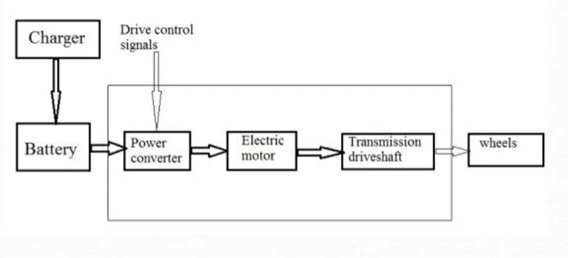
Block Diagram of Electric Vehicle:

Model:

Drive Cycle:

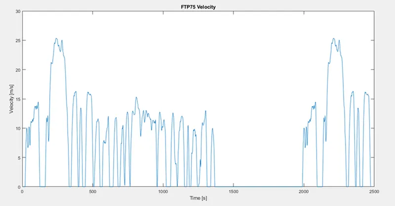
• Below figure we can see the FTP75 drive cycle reference for our vehicle. As per the drive cycle our vehicle runs.
• This drive cycle maximum speed is 25 m/sec and total drive cycle run time is 2474 sec.

Longitudinal Driver:

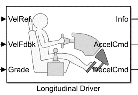
The Longitudinal Driver block implements a longitudinal speed-tracking controller. Based on reference and feedback velocities, the block generates normalized acceleration and braking commands that can vary from 0 through 1. In our case reference velocity is drive cycle and feedback velocity is actual vehicle speed. You can use the block to model the dynamic response of a driver or to generate the commands necessary to track a longitudinal drive cycle. In this model I used the PI control type.

DC Motor:

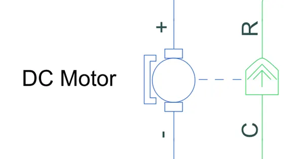
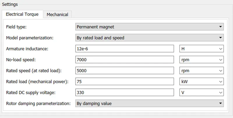
This block represents the electrical and torque characteristics of a DC motor. The block assumes that no electromagnetic energy is lost, and hence the back-emf and torque constants have the same numerical value when in SI units. Motor parameters can either be specified directly, or derived from no-load speed and stall torque. If no information is available on armature inductance, this parameter can be set to some small non-zero value.

H-Bridge:

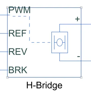
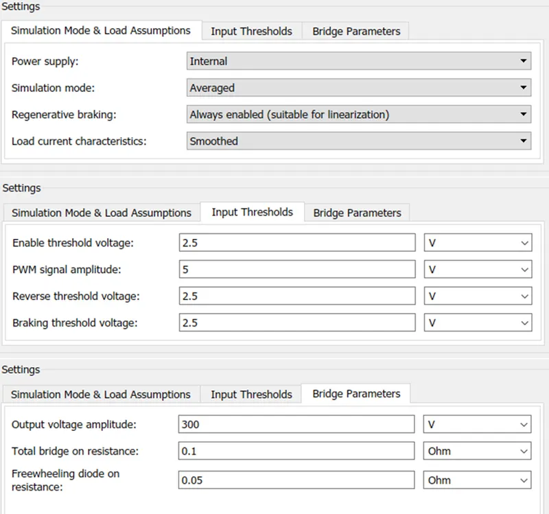
This block represents an H-bridge motor drive. The block can be driven by the Controlled PWM Voltage block in PWM or Averaged mode. In PWM mode, the motor is powered if the PWM port voltage is above the Enable threshold voltage. In Averaged mode, the PWM port voltage divided by the PWM signal amplitude parameter defines the ratio of the on-time to the PWM period. Using this ratio and assumptions about the load, the block applies an average voltage to the load that achieves the correct average load current. The Simulation mode parameter value must be the same for the Controlled PWM Voltage and H-Bridge blocks.

If the REV port voltage is greater than the Reverse threshold voltage, then the output voltage polarity is reversed. If the BRK port voltage is greater than the Braking threshold voltage, then the output terminals are short circuited via one bridge arm in series with the parallel combination of a second bridge arm and a freewheeling diode. Voltages at ports PWM, REV and BRK are defined relative to the REF port.

Controlled PWM Voltage:

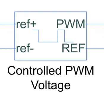
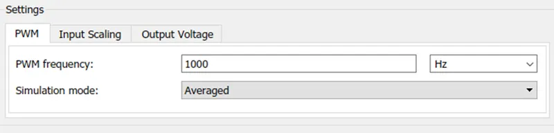
This block creates a Pulse-Width Modulated (PWM) voltage across the PWM and REF ports. The output voltage is zero when the pulse is low, and is equal to the Output voltage amplitude parameter when high. Duty cycle is set by the input value. Right-click the block and select Simscape->Block choices to switch between electrical +ref/-ref ports and PS input u to specify the input value.

At time zero, the pulse is initialized as high unless the duty cycle is set to zero or the Pulse delay time is greater than zero.

The Simulation mode can be set to PWM or Averaged. In PWM mode, the output is a PWM signal. In Averaged mode, the output is constant with value equal to the averaged PWM signal

Vehicle Body:

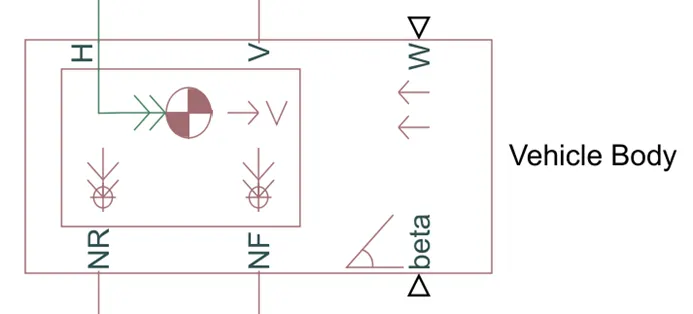
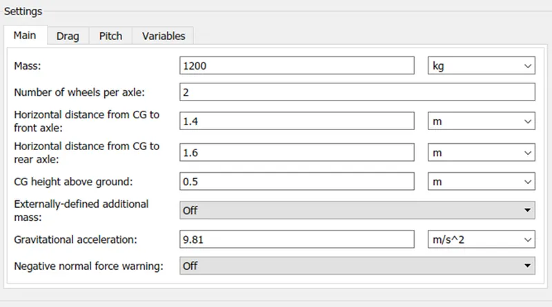
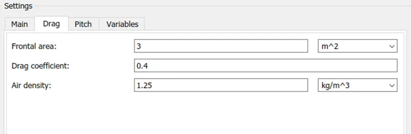
The Vehicle Body block represents a two-axle vehicle body in longitudinal motion. The vehicle can have the same or a different number of wheels on each axle. For example, two wheels on the front axle and one wheel on the rear axle. The vehicle wheels are assumed identical in size. The vehicle can also have a center of gravity (CG) that is at or below the plane of travel.

The block accounts for body mass, aerodynamic drag, road incline, and weight distribution between axles due to acceleration and road profile. Optionally include pitch and suspension dynamics. The vehicle does not move vertically relative to the ground.

The block has an option to include an externally-defined mass and an externally-defined inertia. The mass, inertia, and center of gravity of the vehicle body can vary over the course of simulation in response to system changes.

Tire:

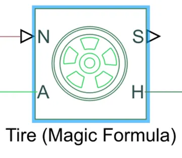
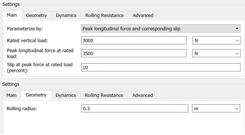
Represents the longitudinal behavior of a highway tire characterized by the tire Magic Formula. The block is built from Tire-Road Interaction (Magic Formula) and Simscape Foundation Library Wheel and Axle blocks. Optionally, the effects of tire inertia, stiffness, and damping can be included.

Simple Gear:

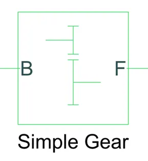
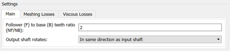
The Simple Gear block represents a gearbox that constrains the connected driveline axes of the base gear, B, and the follower gear, F, to corotate with a fixed ratio that you specify. You choose whether the follower axis rotates in the same or opposite direction as the base axis. If they rotate in the same direction, the angular velocity of the follower, ωF, and the angular velocity of the base, ωB, have the same sign. If they rotate in opposite directions, ωF and ωB have opposite signs.

SOC Estimate Subsystem:

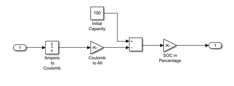
The subsystem determines the state of charge remaining in the battery by using some math function and constant blocks. The below figure shows inside the SOC Estimate subsystem.

Vehicle Subsystem:

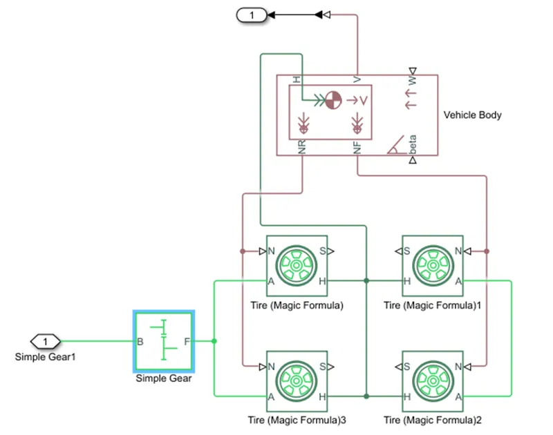
This subsystem consists of the vehicle body, tire and simple gear blocks. It delivers the motor output power to the wheel. The below figure shows inside the vehicle subsystem.

Simulink Model Step:

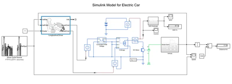
• First I created a vehicle subsystem as you see in the earlier figure and DC motor mechanical power output connected to the simple gear. At the same time, the DC motor is controlled by the H-bridge and Controlled PWM Voltage.
• Controlled PWM voltage is controlled by the longitudinal driver through the controlled voltage source.
• For reference velocity gives drive cycle source FTP75 to the longitudinal driver and similarly actual velocity as a feedback velocity.
• Measure the DC motor current and calculate the remaining SOC of the battery by using the SOC Estimate subsystem.
• Similarly, calculate the distance traveled by car by integrating the actual speed of the car and dividing 1000 for transfer meter to Kilometers.

Results:

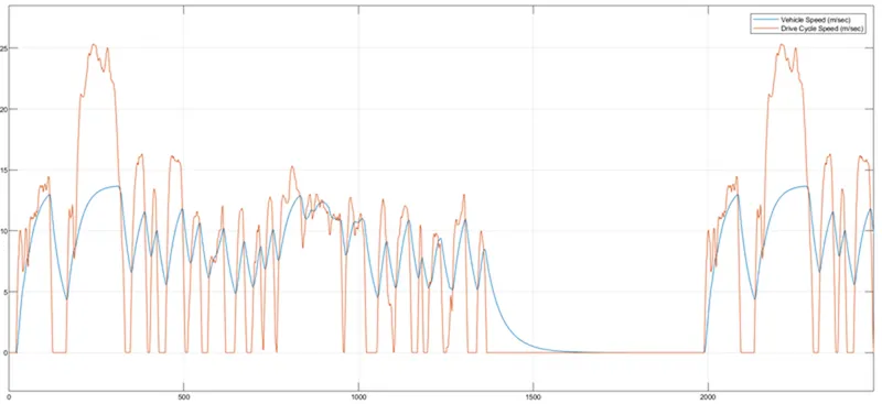
• The above figure shows the car speed and drive cycle speed. At some point its overlaps to each other but at some time is a mismatch.
• But they overlapped with each other to complete drive cycle time. They are not because of some motor power and current limitations.
• The below figure shows the remaining SOC in the battery and another figure shows the DC motor current.

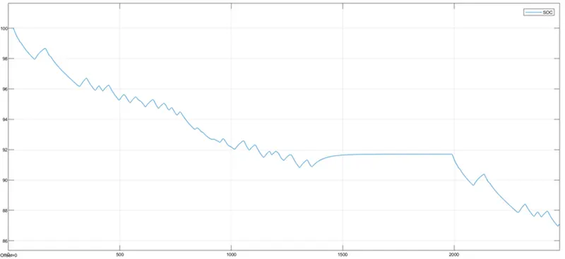
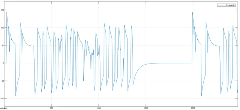
• After completing the simulation, the remaining SOC is 87.12% and the travel distance by the car is 17.25 Km for FTP75 drive cycle.
• We can see that current is fluctuated as per drive cycle requirement. When speed is increased current is positively increased and when speed decreases current also decreases and goes negative.
• If you compare the current graph with the SOC graph you can observe, when current is positive SOC is decreased, but when current goes negative SOC is slightly increased. It's called regenerative braking.

Conclusion:

• Created a simulation model for an electric car, during that I worked on some interesting blocks like H-bridge, Controlled PWM Voltage, Vehicle body, etc.
• Also I observed SOC estimation, regenerative braking, DC motor control, Vehicle architecture.