Exhaust Port Challenge
Aim
Aim of this challenge is understand the conjugate heat transfer type problem and run the simulation of exhaust port of engine.
- Give a brief description of why and where a CHT analysis is used.
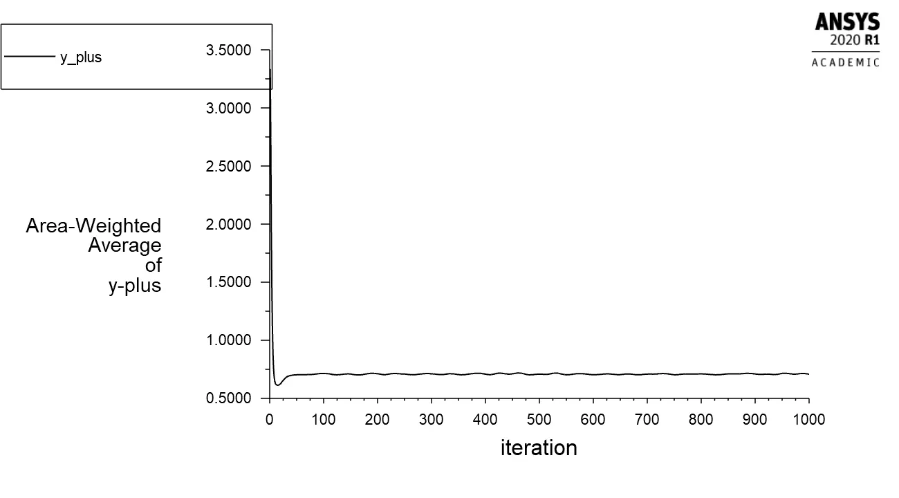
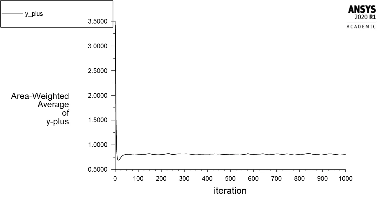
- Maintain the y+ value according to the turbulence model and justify the results.
- Calculate the wall/surface heat transfer coefficient on the internal solid surface & show the velocity & temperature contours in appropriate areas.
- How would you verify if the HTC predictions from the simulations are right? On what factors does the accuracy of the prediction depend on?
Part-1:
Give a brief description of why and where a CHT analysis is used.
The term conjugate heat transfer (CHT) is used to describe processes which involve variations of temperature within solids and fluids, due to thermal interaction between the solids and fluids. The exchange of thermal energy between the two physical bodies is called study of Heat Transfer, the rate of transferred heat is directly proportional to the temperature difference between the bodies. A typical example is the heating or cooling of a solid object by the flow of air in which it is immersed and some other example includes conduction through solids, free and forced convection in the gases/fluids and thermal radiation.Typical applications of this analysis type exist as, but are not limited to, the simulation of heat exchangers, cooling of electronic equipment, and general-purpose cooling and heating systems.
Conjugate heat transfer corresponds with the combination of heat transfer in solids and heat transfer in fluids. In solids, conduction often dominates whereas in fluids, convection usually dominates. Efficiently combining heat transfer in fluids and solids is the key to designing effective coolers, heaters, or heat exchangers. Forced convection is the most common way to achieve high heat transfer rate. In some applications, the performances are further improved by combining convection with phase change (for example liquid water to vapor phase change).
Heat transfer in solids and heat transfer in fluids are combined in the majority of applications. This is because fluids flow around solids or between solid walls, and because solids are usually immersed in a fluid.
Modes of heat transfer
- Conduction: diffusion of heat due to temperature gradients. A measure of the amount of conduction for a given gradient is the heat conductivity.
- Convection: when heat is carried away by moving fluid. The flow can either be caused by external influences, forced convection; or by buoyancy forces, natural convection. Convective heat transfer is tightly coupled to the fluid flow solution.
- Radiation: transfer of energy by electromagnetic waves between surfaces with different temperatures, separated by a medium that is at least partially transparent to the (infrared) radiation. Radiation is especially important at high temperatures, e.g. during combustion processes, but can also have a measurable effect at room temperatures.
An accurate description of heat transfer modes, material properties, flow regimes, and geometrical configurations enables the analysis of temperature fields and heat transfer.
Typical design problems involve the determination of:
- Overall heat transfer coefficient, e.g. for a car radiator.
- Highest (or lowest) temperature in a system, e.g. in a gas turbine, chemical reaction vessels, food ovens.
- Temperature distribution (related to thermal stress), e.g. in the walls of a spacecraft.
- Temperature response in time dependent heating/cooling problems, e.g. engine cooling, or how fast does a car heat up in the sun and how is it affected by the shape of the windshield?
The fluid flow and heat transfer problems can be tightly coupled through the convection term in the energy equation and when physical properties are temperature dependent. While analytical solutions exist for some simple problems, we must rely on computational methods to solve most industrially relevant applications.
CHT can be performed to improve cooling performance of the water jacket and increase engine life. Advancements in cooling for applications such as gas turbines components require improved understanding of the complex heat transfer mechanisms and the interactions between those mechanisms, which our engineers can perform without hassle. Critical cooling applications often rely on multiple thermal protection techniques, including internal cooling, external film cooling, etc. which are efficiently used by our analysis to cool components and limit the use of coolant. We do extensive support for Motor and Battery CHT Analysis to get optimized design for High voltage systems. Conjugate Heat Transfer analysis provides the temperature distribution in solid and coolant of the engine and clear insight on velocity distribution and mechanism of heat transfer of coolant. Results of CHT analysis become input to structural simulations as thermal loads.
We have a wide experience in Engine CHT Analysis for various type of engines like Bikes, Passenger Cars, Racing cars, Commercial Vehicles, Marine, Agricultural equipment and Earth-moving equipment etc.
Mathematical Modeling
The flow of thermal energy from matter occupying one region in space to matter occupying a different region in space is known as heat transfer. Heat transfer can occur by three main methods:
- Conduction
- Convection
- Radiation
Physical models involving conduction and/or convection only are the simplest while buoyancy-driven flow or natural convection and radiation models are more complex. Depending on your problem, ANSYS Fluent will solve a variation of the energy equation that takes into account the heat transfer methods you have specified.
- Modeling Conductive and Convective Heat Transfer
ANSYS Fluent allows you to include heat transfer within the fluid and/or solid regions in your model. Problems ranging from thermal mixing within a fluid to conduction in composite solids can therefore be handled by ANSYS Fluent. When your ANSYS Fluent model includes heat transfer you will need to activate the relevant physical models, supply thermal boundary conditions, and input material properties that govern heat transfer and/or vary with temperature as part of the setup.
ANSYS Fluent solves the energy equation in the following form:
`frac{partial (rho E) }{partialt}+ nabla.(v(rhoE+p)) = nabla .(k_(eff)nablaT-sumh_jJ_j+(tau_(eff).v))+s_h` (1.1)
where `k_(eff)`is the effectivity conductivity (`k+k_t`, where `k_t`is the turbulent thermal conductivity, defined according to the turbulent model being used), `J_j`is the difusion flux of species j. The first three terms on the right hand side of eq(1.1) represent energy transfer due to conduction, species diffusion, and viscous dissipation, respectively. `S_h` includes the heat of chemical reaction, and any other volumeric heat sources you have defined.
In equation(1.1) `E=h-frac{p}{rho}+frac{v^2}{2}` (1.2)
Where sensible enthalpy h is defined for ideal gases as `h=sumY_jh_j` (1.3)
and for incompressible flow as `sumY_jh_j+frac{p}{rho}` (1.4)
In equation (1.3) and (1.4), `Y_j` is the mass fraction of the species j and `h_j=int_(ref)^Tc_(p,j)dT`
The value used for `T_(ref)`in the sensible enthalpy calculation depends on the solver and models in use. For the pressure based solver `T_(ref)` is 298.15 K except for PDF models in which case `T_(ref)`is a user input for the species. For the density-based solver `T_(ref)`is 0 k except when modelling species transport with reactions in which case `T_(ref)` is a user input for the species.
Part-2
CHT analysis on a model of a exhaust manifold
- Geometry preparation
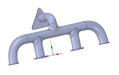
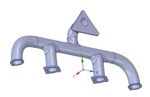
- Geometrtry of exhaust manifold
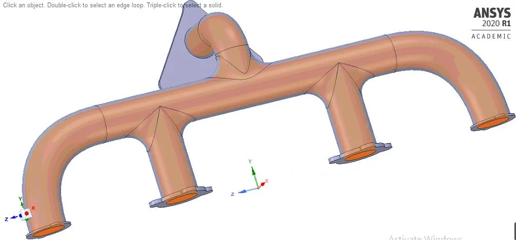
First of all importe the geometry of exhaust manifold in the space claim. This is the solid body model of the exhaust port manifold. The material for this model is aluminum.
- Extract fluid volume by selecting edges
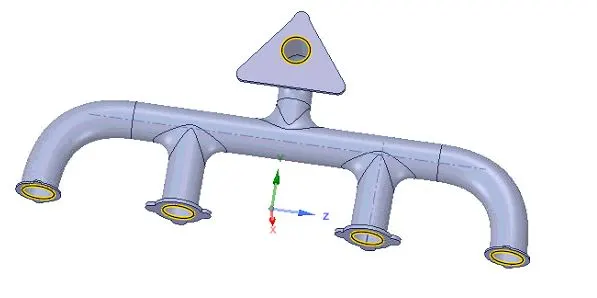
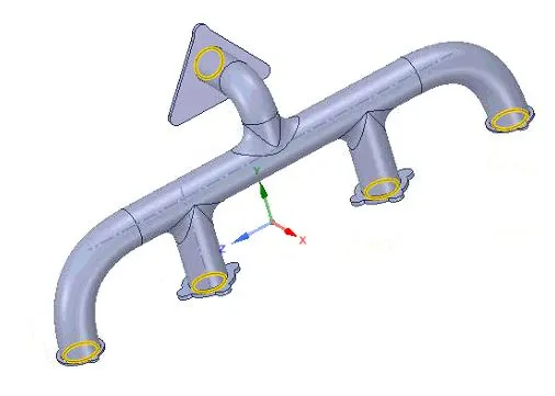
In order to define the fluid volume 4 edges of inlets and one edge of outlet is selected.
- Extracted fluid volume
This is the extracted flhid volume where the fluid flows. The given below figure represent the fluid region inside the exhaust port manifold. Consider the 4 ports as inlet combining to a single outlet. The velocity of the inlet fluid is 5 m/s and with temperature of 700K.
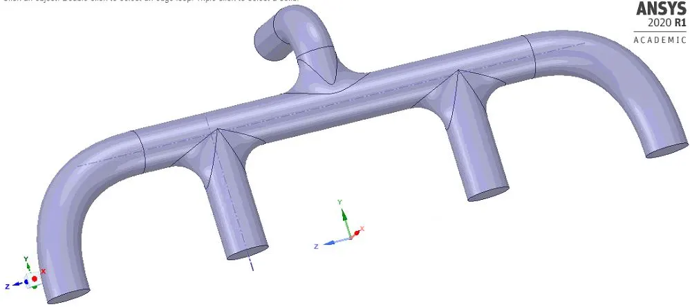
- Fluid volume inside the solid volume
- Sharing topology of the geometry
In order to capture the conjugate heat transfer the solids and fluids regions, both solid and fluid should share the properties which could be done by enabling the share topology option. The pink colour edges and yellow faces shows which information is being shared with both solid and fluid volumes. This also work to obtain the conformal mesh.
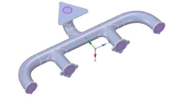
- Case-1 Base line mesh simulation
- Name selection
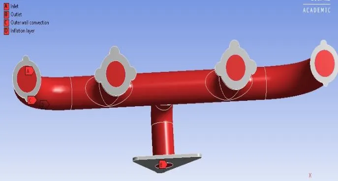
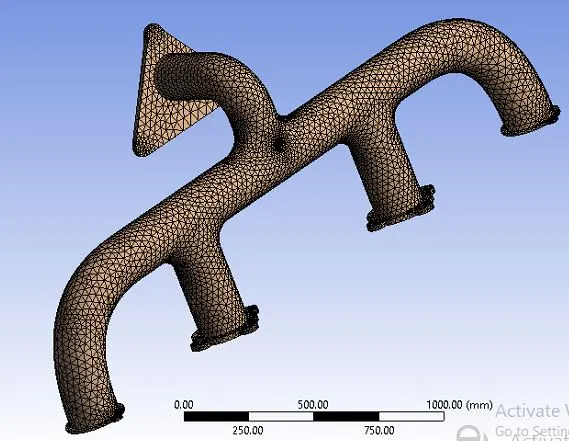
- Base line mesh setting
- Elemeny size: 150 mm
- No of nodes: 27472
- No of elements: 137732
- Confirmal Mesh
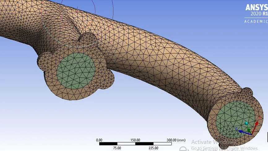
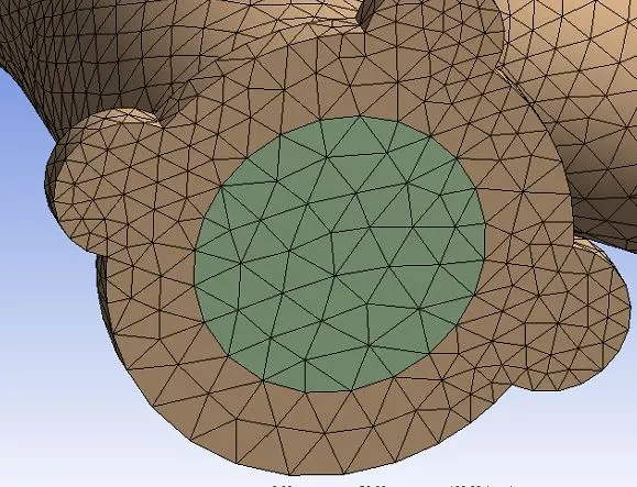
Faces and vortex are perfectly coinciding.
Fluent Case-setup
- Time: Steady state
- Solver type: pressure based
- Velocity formulation: absolute
- Viscous model:
Model: K-omega
K-Omega: SST
Option : production limiter
- Material type: For fluid volume: air,
For solids : aluminium
- Boundary conditions
- Inlet = type(velocity inlet) = 5 m/s and temperature of air = 700K
- Outer wall convection = Thermal convection with heat transfer coefficient is 20`W/m^2 K`
- Outlet: Pressure outlet
- We use the hybrid initialization.
- Post processing: we set the temperature contours and animation of temperature.
Results
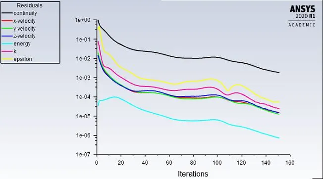
Residuals
Temperature contours
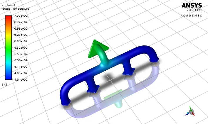
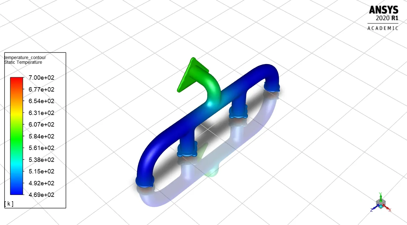
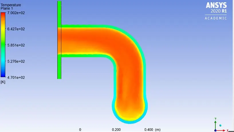
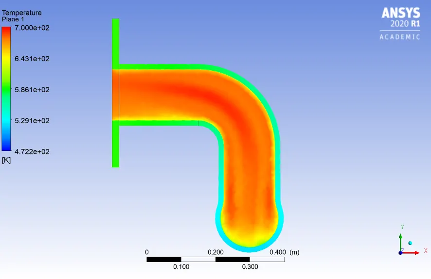
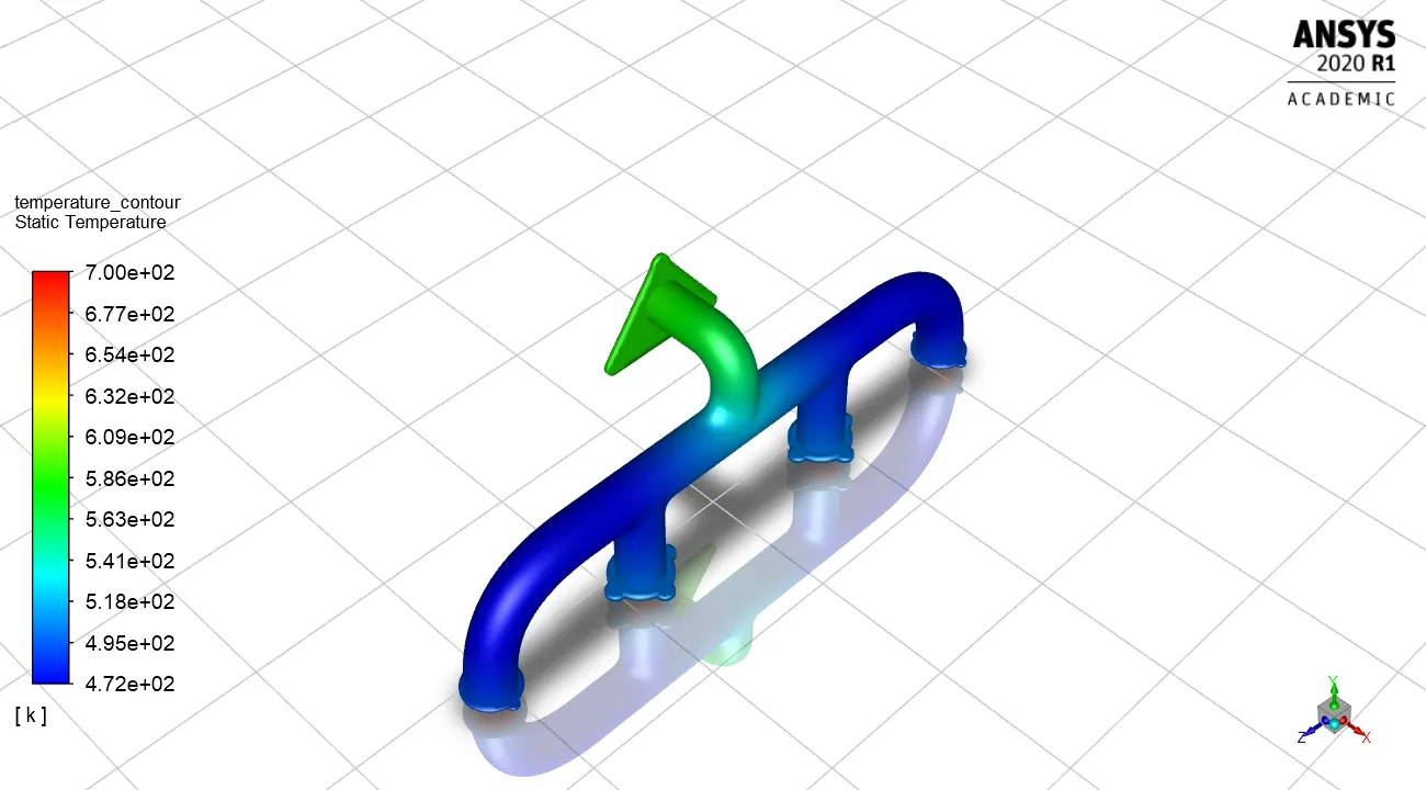
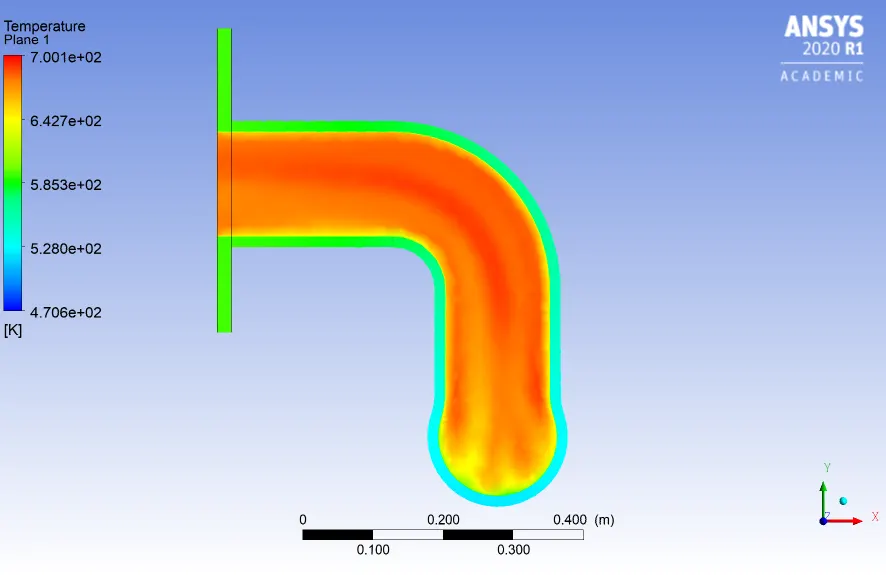
In the above image we observe that the temperature is starting too much high at the joint. Because at that point velocity is too much high and temperature of the hot air is increased.
Velocity contours
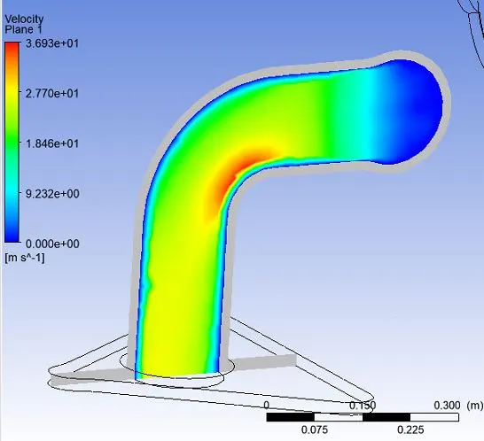
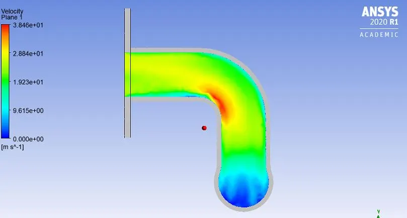
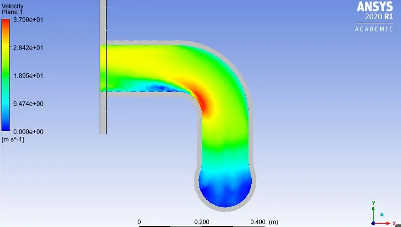
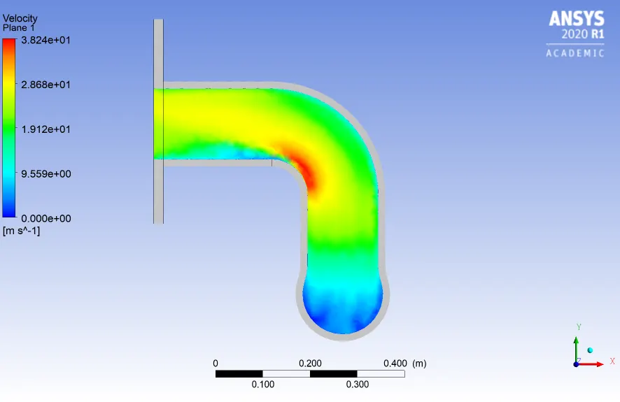
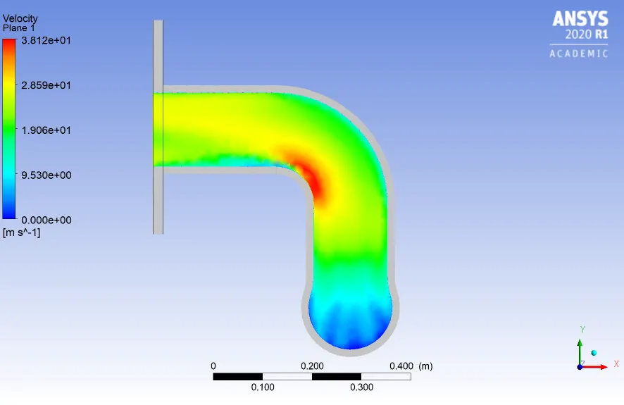
In the above image we easily observe that at the elbow velocity is too much.
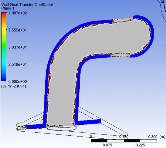
Wall heat transfer coefficient
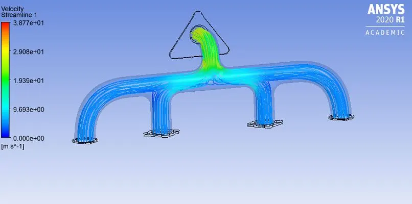
Streamlines
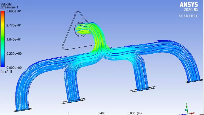
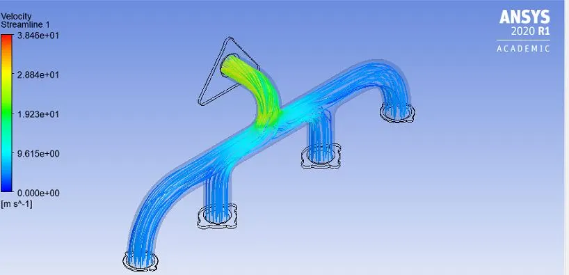
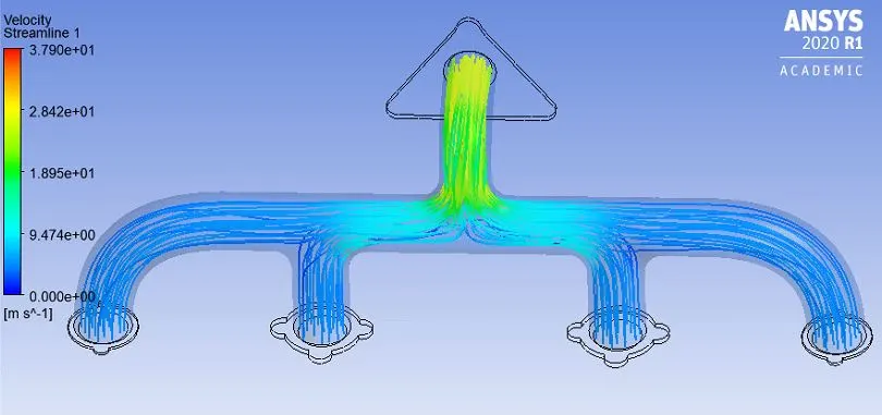
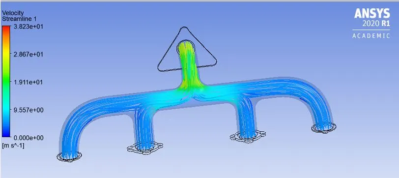
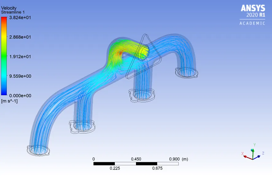
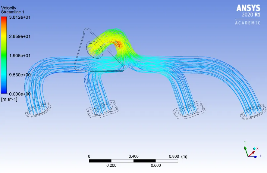
In the above image we easily observe that at the point where all the pipes are join together velocity is going to increase.
Q.2. Maintain the y+ value according to the turbulence model and justify the results.
First layer thickness calcuation
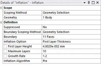
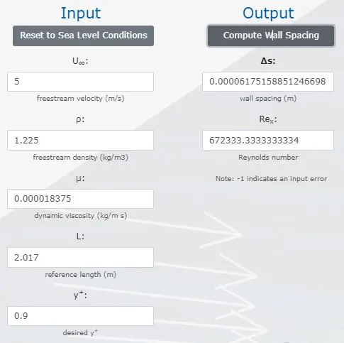
- I have use the following values for the calculation of first layer thickness. Value of first layer thickness has a too much impact on the the results and also it is too much technical to adjust this value according to problem nature.
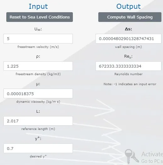
- Meshing details by using the value of y_plus=0.7 with coarse mesh
- Inflation layers on fluid body
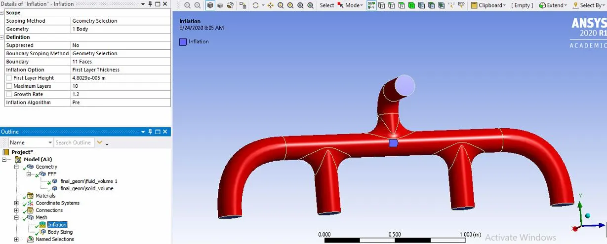
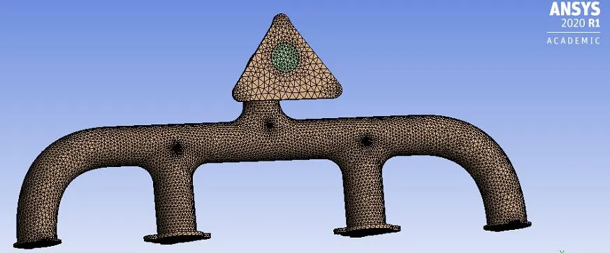
- Mesh

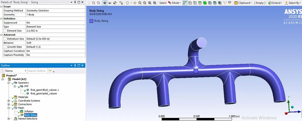
- Body sizing on the fluid zone
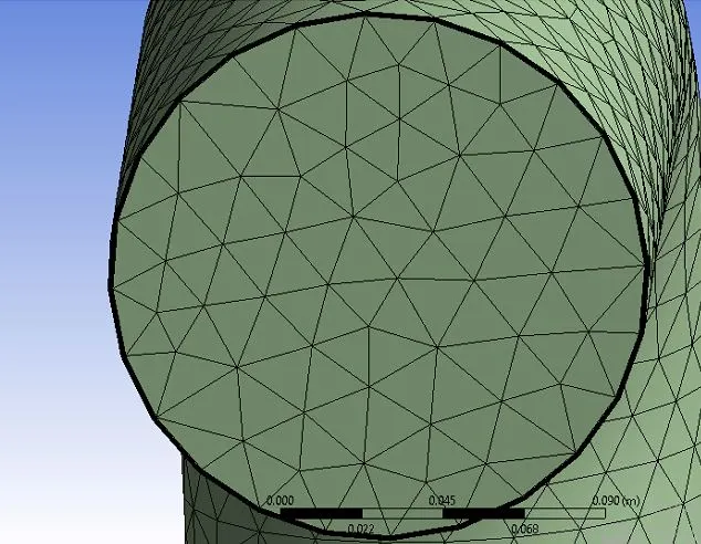
- Mesh on fluid body
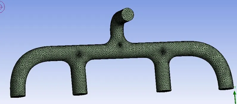
- Overall mesh details Solid body mesh
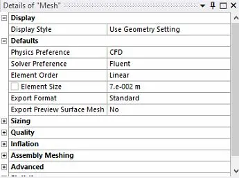
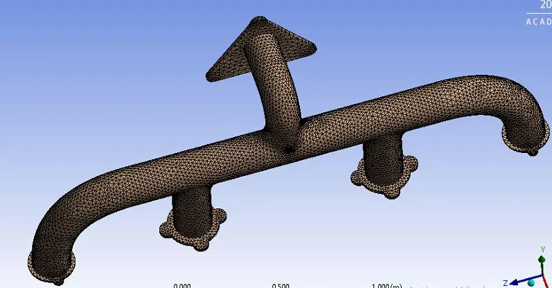
Mesh Statistics
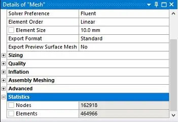
Results
Residuals
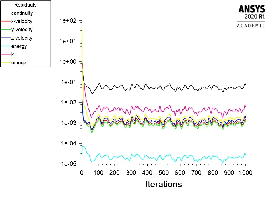
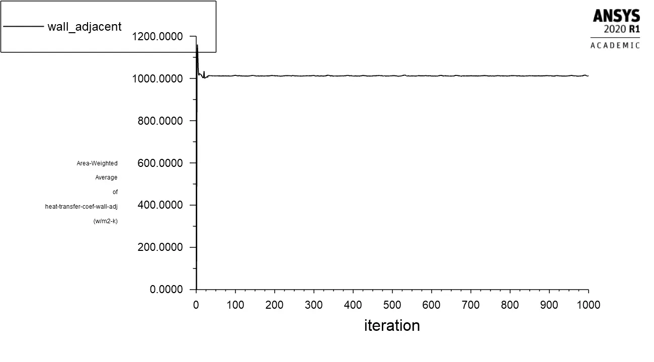
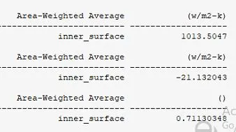
Wall heat transfer coefficient
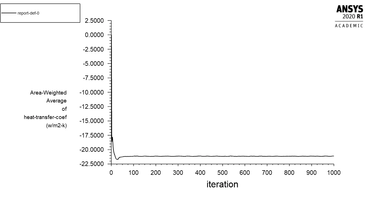
Surface heat transfer coefficient
Y-plus
Temperature Contours
Streamlines
Velocity Contours at plane
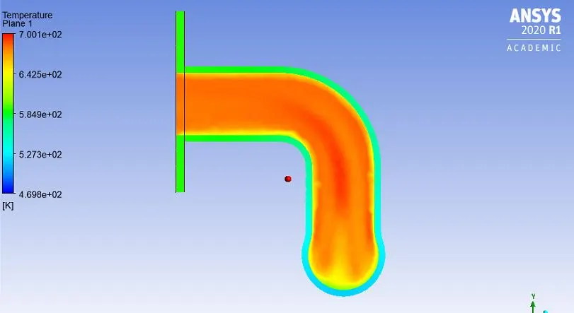
Temperature Contours at plane
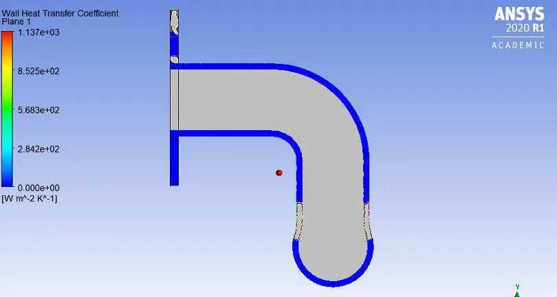
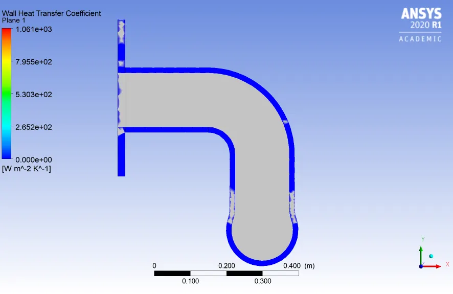
Wall heat transfer coefficient at plane
- With the same 0.7 Y_plus value, run the simulation with 443147 elements(Refine mesh)
- Note:
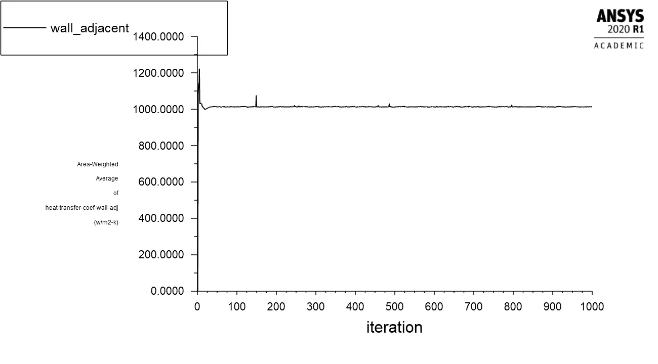
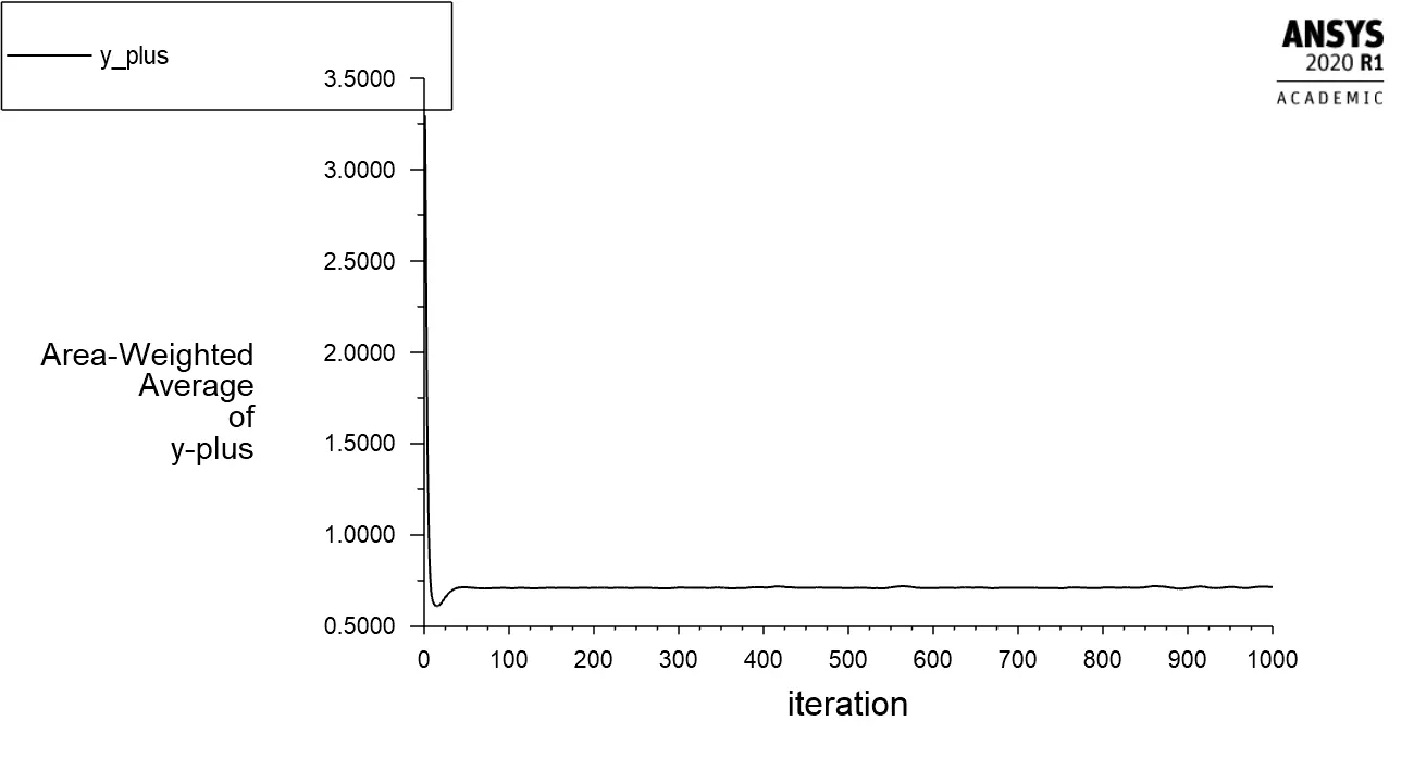
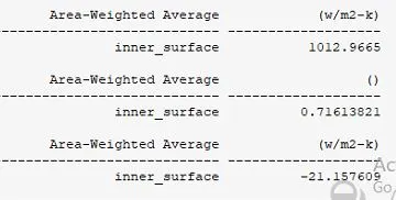
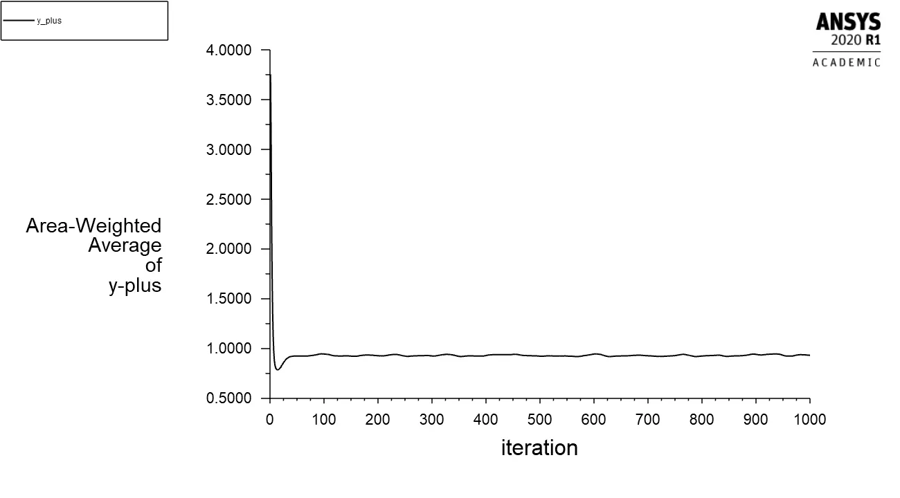
There is not too much change occur in the results. The value of wall heat transfer, surface heat transfer coefficients and the range of the y_plus is also same as in the coarse case.
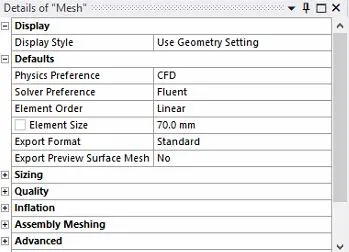
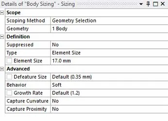
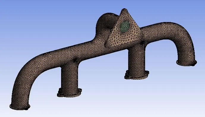
- Mesh details:

- Results
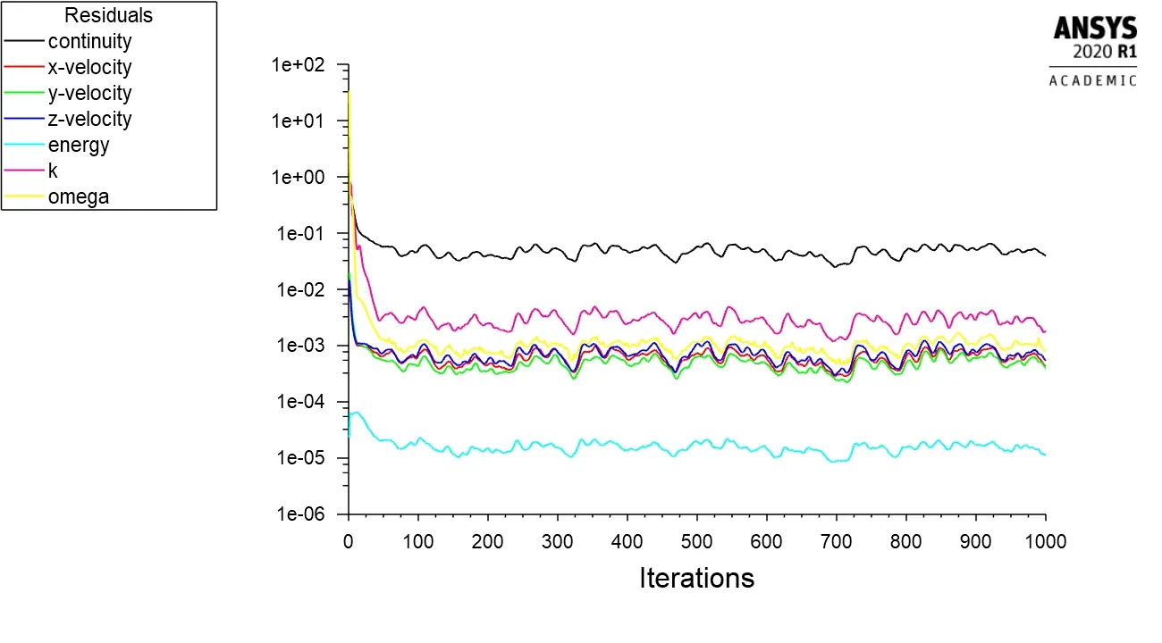
Residuals
Wall heat transfer coefficient
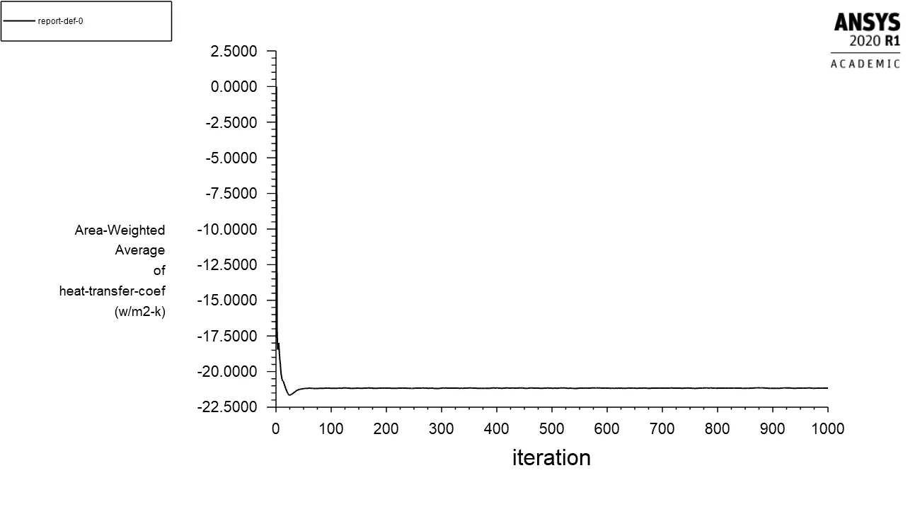
Surface heat transfer coefficient
Y_plus
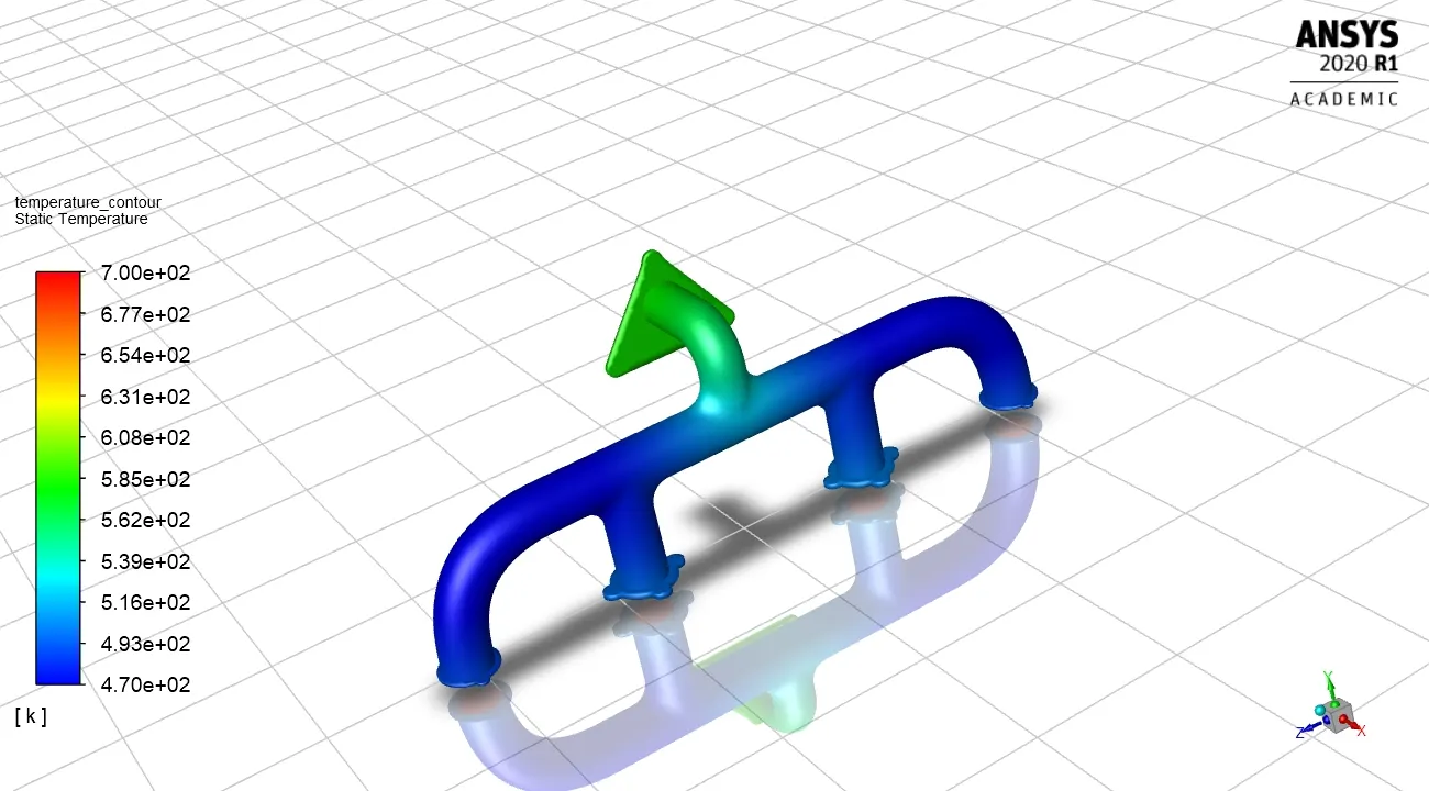
Temperature Contours
Stream lines
Velocity Contours at plane
Temperature Contours at plane
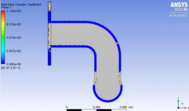
Wall heat transfer coefficient
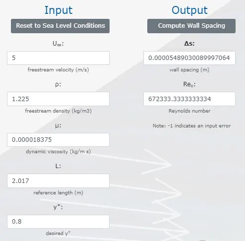
First layer thickness with 0.8 Y_plus
- With the same 0.8 Y_plus value, run the simulation with 443147 elements
- Note:
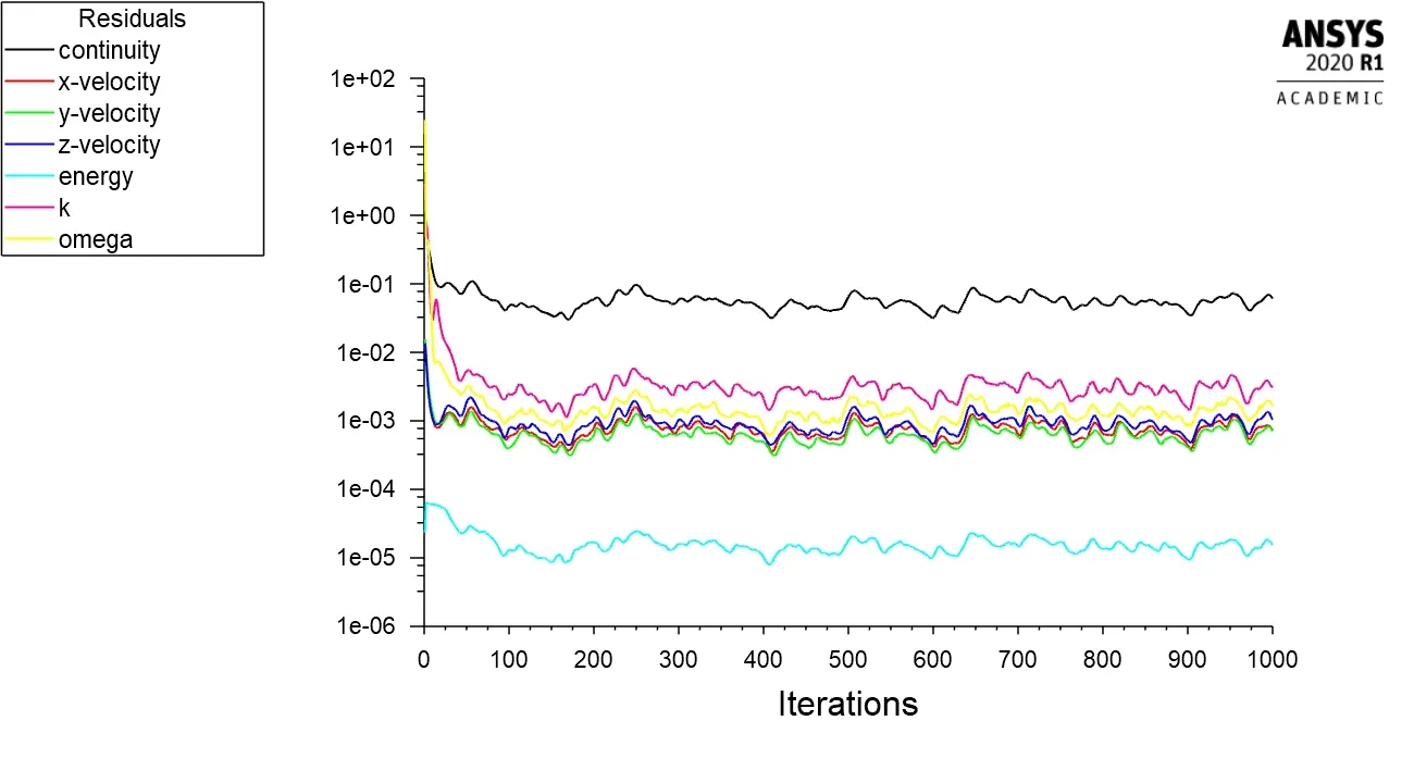
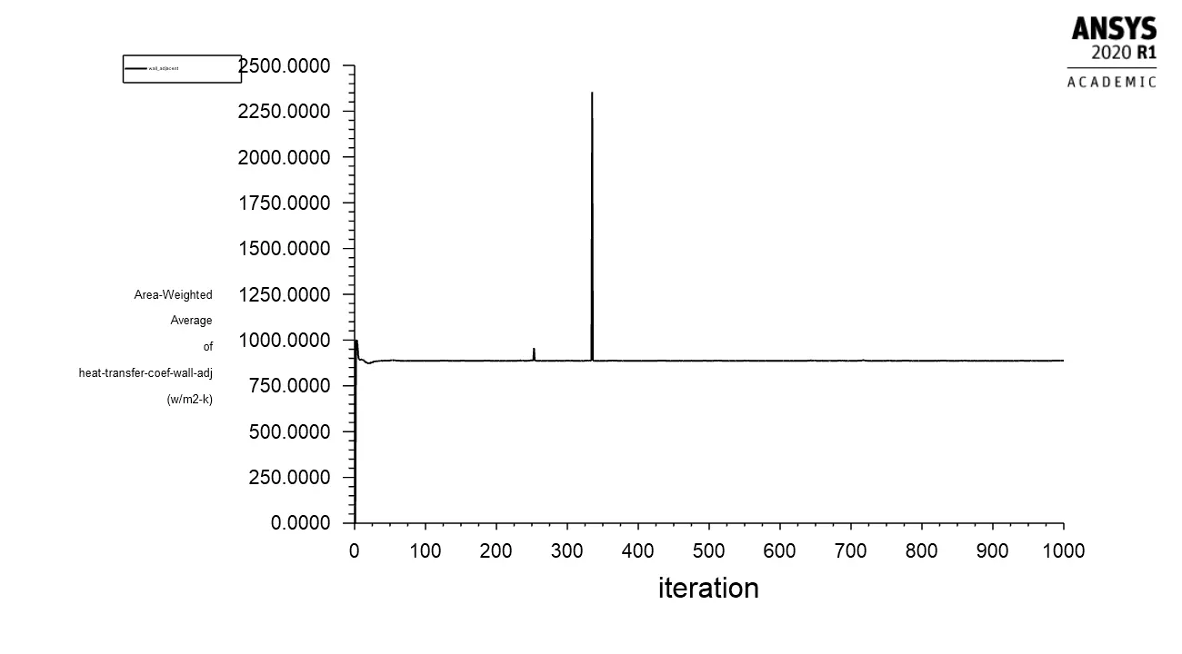
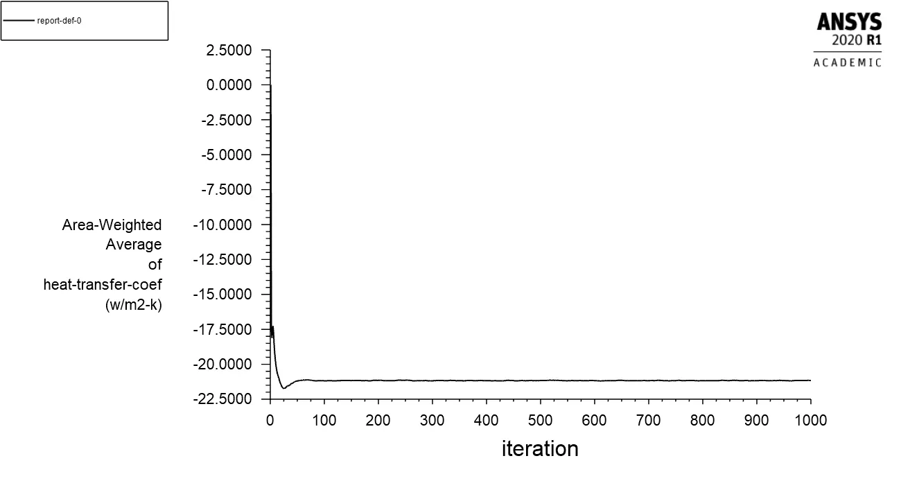
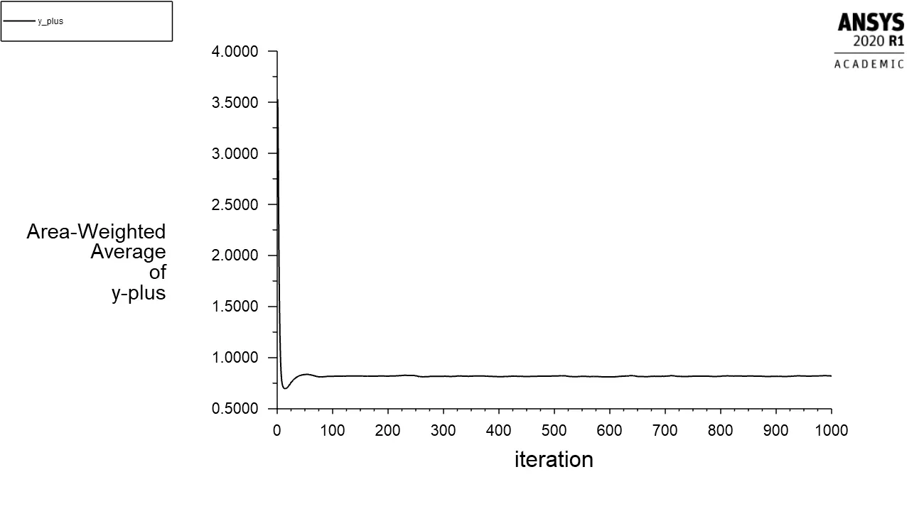
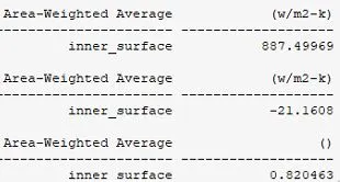
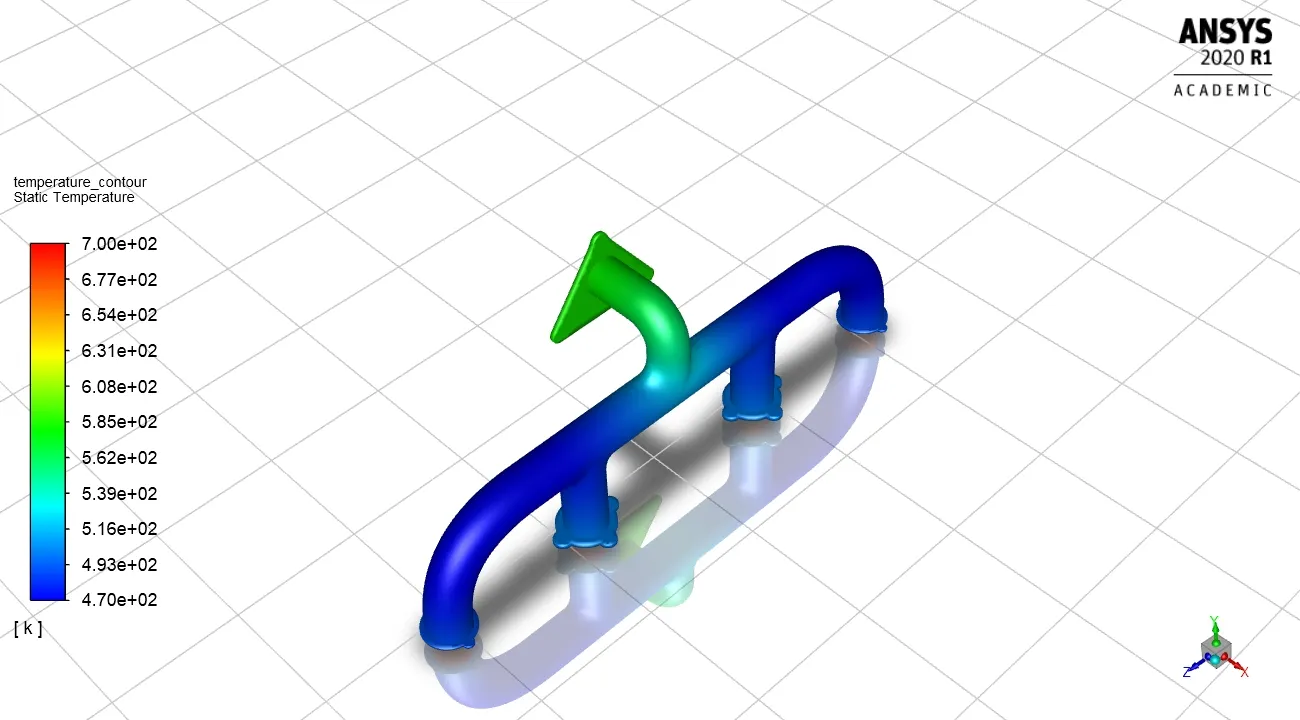
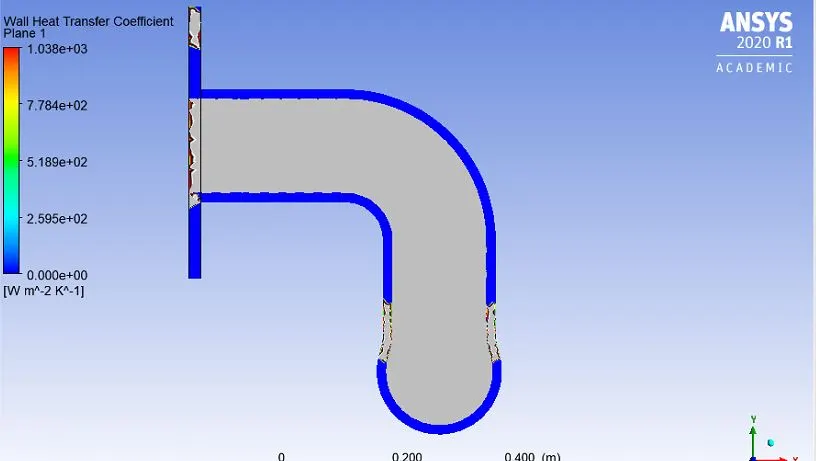
There is a change occur in the results. The value of wall heat transfer, surface heat transfer coefficients and the range of the y_plus are changed by changing the value of Y_plus.
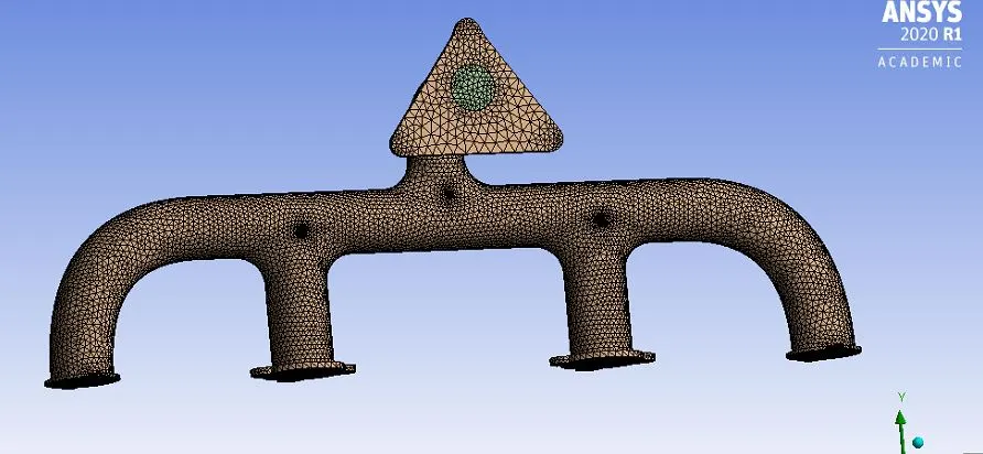
Mesh details:

Results
Residuals
Wall heat transfer coefficient
Surface heat transfer coefficient
Y_plus
Temperature Contours
Streamlines
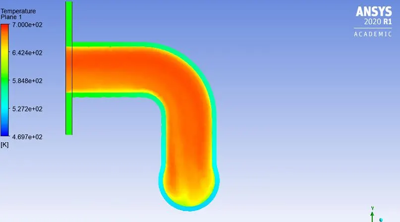
Temperature Contours at plane
Velocity Contours at plane
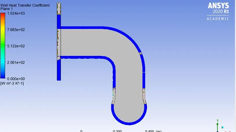
Wall heat transfer coefficient
First layer thickness with 0.79 Y_plus
- With the same 0.79 Y_plus value, run the simulation with 443147 elements
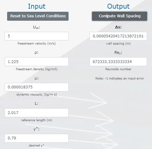
Mesh Details

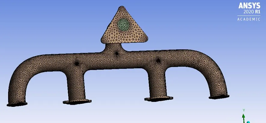
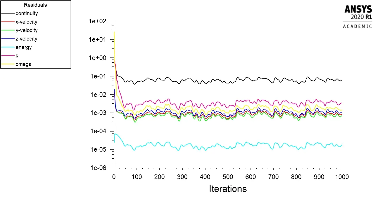
Results
Residuals
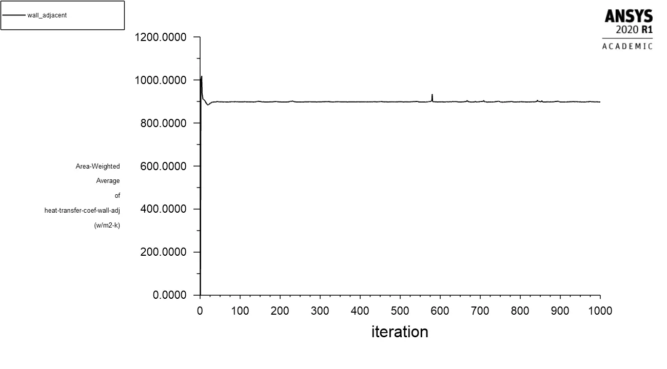
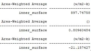
Wall heat transfer coefficients
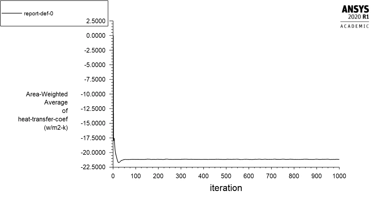
Surface heat transfer coefficients
Y_plus
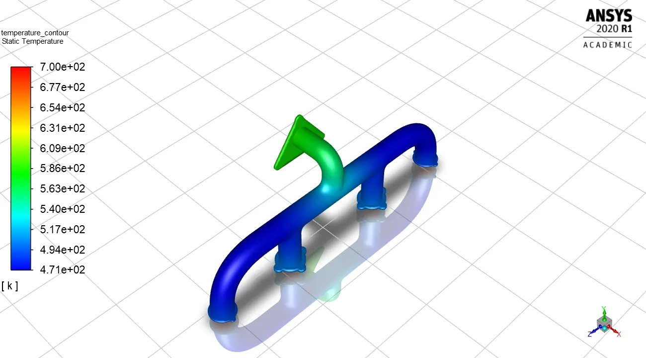
Temperature Contours
Streamlines
Temperature contours at plane
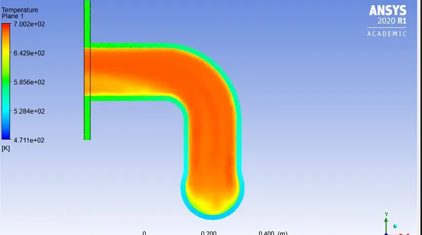
Velocity Contours at plane
Wall Heat transfer coefficient
First layer thickness with 0.76 Y_plus
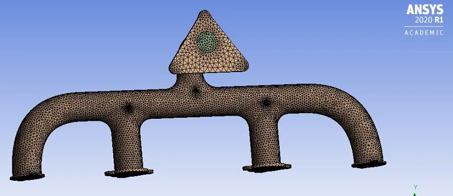
- With the same 0.76 Y_plus value, run the simulation with 443357 elements
Mesh Details

Results
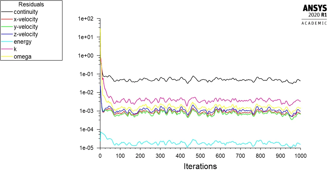
Residuals
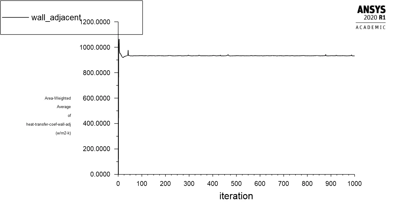
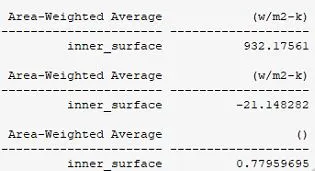
Wall heat transfer coefficient
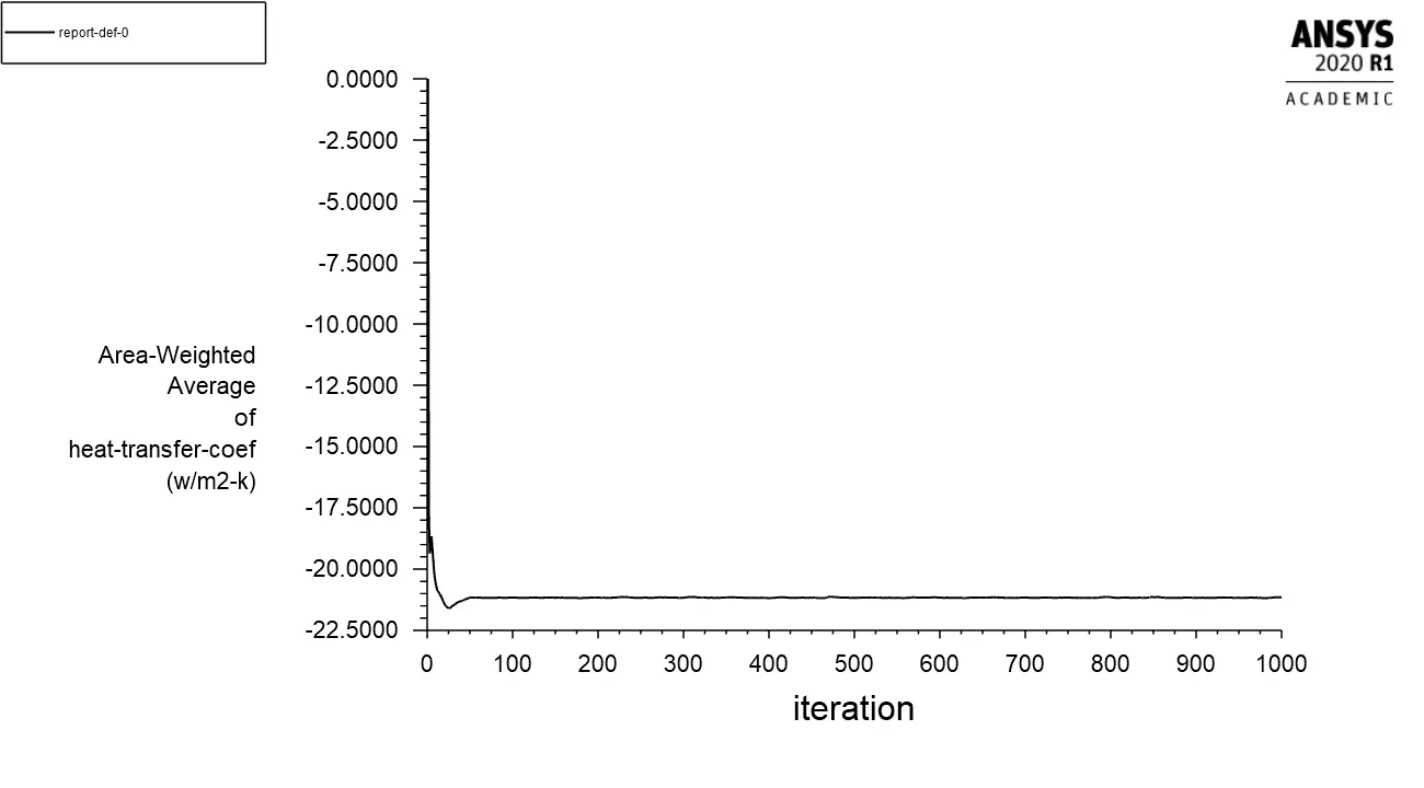
Surface heat transfer coefficient
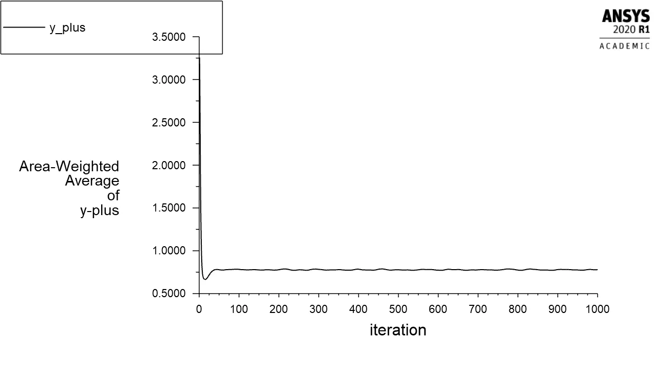
Y_plus
First layer thickness with 0.9 Y_plus
- With the same 0.9 Y_plus value, run the simulation with 442513 elements
Mesh Details

Results
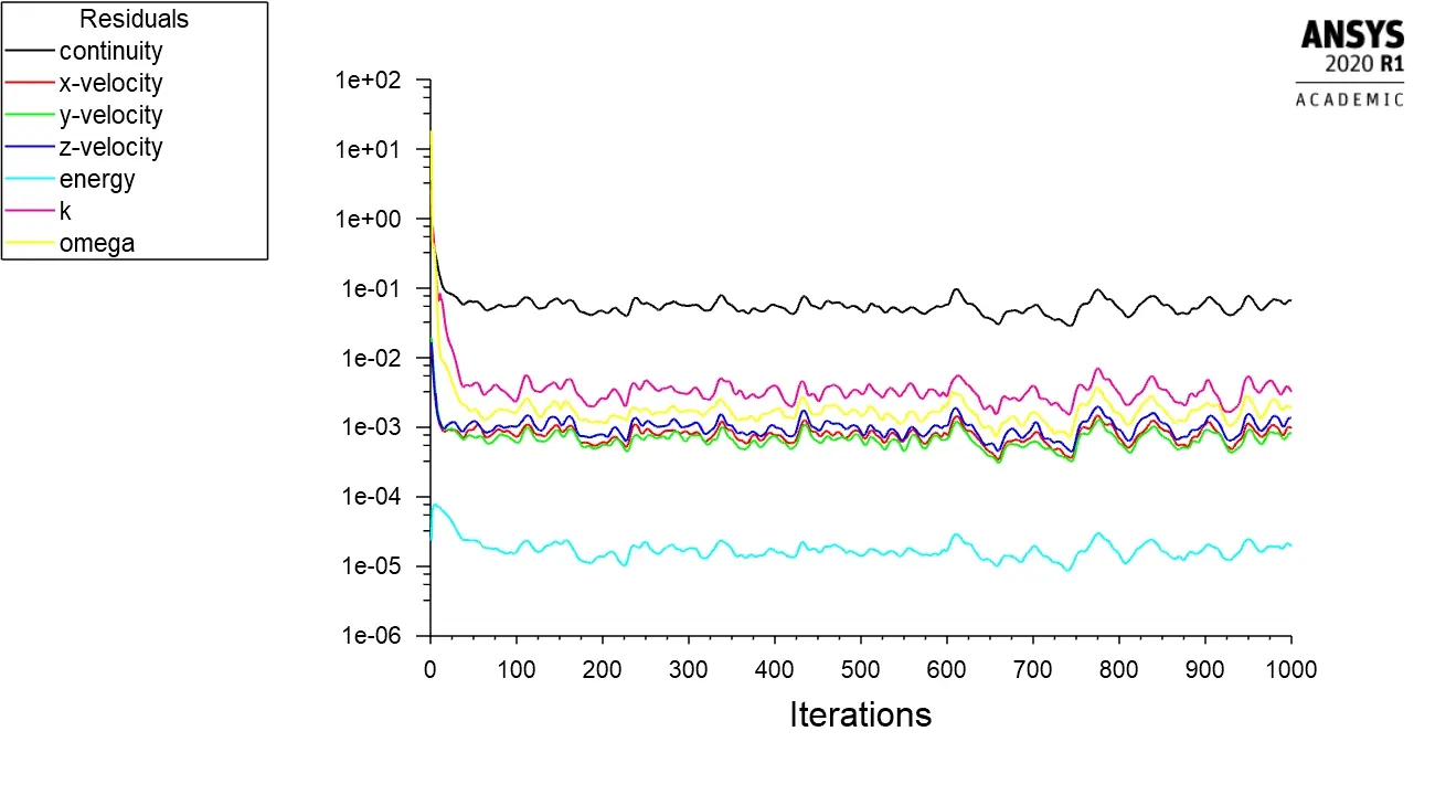
Residuals
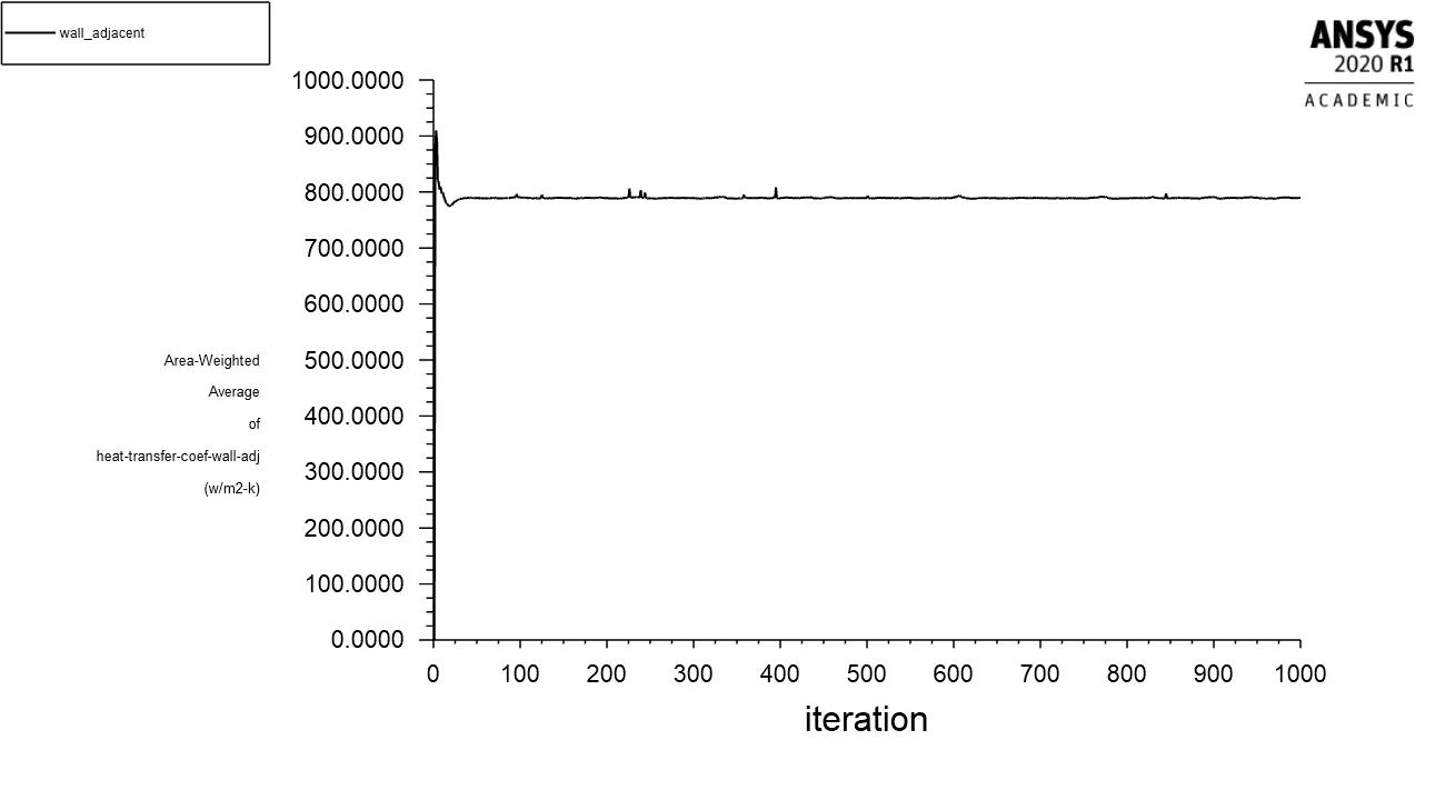
Wall heat transfer coefficient
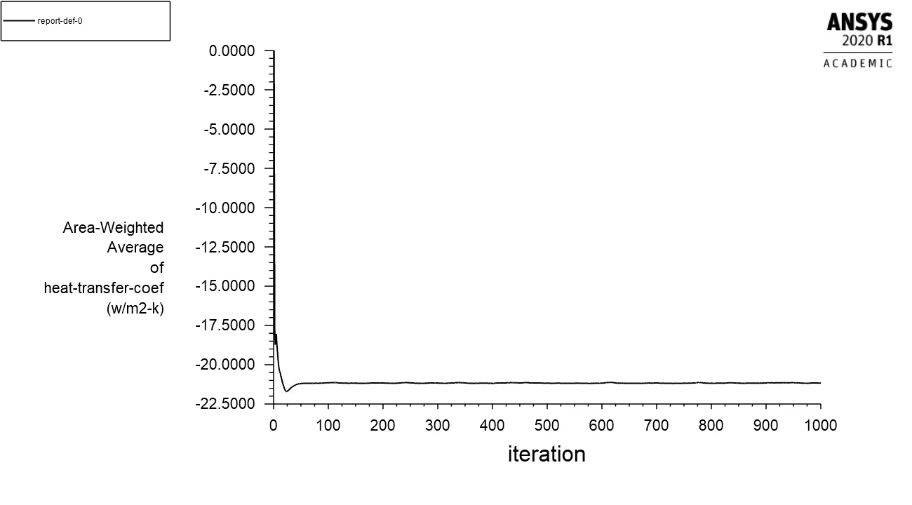
Surface heat transfer coefficient
Y_plus
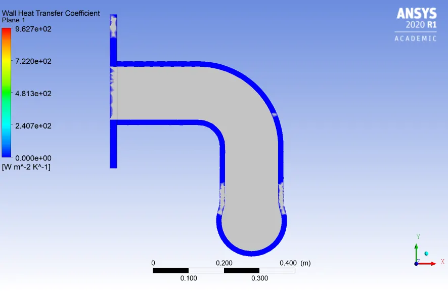
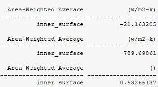
Results discussions
| Y-plus value | First layer thickness value | Wall Heat transfer value | Surface Heat transfer value |
| 0.7 | 0.000048029013287 | 1013.5047 | -21.132043 |
| 0.76 | 932.17561 | -21.148282 | |
| 0.79 | 0.000054204172138 | 897.74758 | -21.157427 |
| 0.80 | 0.000054890300899 | 887.49969 | -21.1608 |
| 0.90 | 0.0000617515885124 | 789.69861 | -21.163205 |
Q.4. How would you verify if the HTC predictions from the simulations are right? On what factors does the accuracy of the prediction depend on?
Heat transfer coefficient is a quantitative characteristic of convective heat transfer between a fluid medium (a fluid) and the surface (wall) flowed over by the fluid. One way is to verify the simulation results using the mesh independency test. In this project we also did the mesh independency test and in a finer mesh we almost got the same values of wall and surface heat transfer coefficients.
On what factors does the accuracy of the prediction depend on?
1. Value of surface and wall heat transfer coefficient are depend on the mesh quality.
2. Finer mesh give the more accurate value.
3. And also the value of Y-plus in the calculation of first layer thickness is also play an very important role.
4. No of inflation layers is also play an important role.
5.Mesh should be conformal for smoothing transferring of mesh in different zone.
References:
1.V M Latheesh, P Parthasarathy, V Baskaran and S Karthikeyan, "Design and CFD analysis of intake port and exhaust port for a 4 valve cylinder head engine".
2. Marupilla Akhil Teja, Katari Ayyappa, Sunny Katam and Panga Anusha, "Analysis of Exhaust Manifold using Computational Fluid Dynamics".