Evaluation of ATV model in SIMULINK

Aim: To carry out a system level simulation of the all-terrain vehicle.

Description:

In this project, we have a model that simulate the working of the BAJA all-terrain vehicle. The model shows how to build an ATV with CVT which is mostly used in BAJA vehicle. Simscape and Simscape Driveline have been used to complete the system. The engine data used in the model is provided as an image which shows the Engine Speed (RPM) vs Torque curve.

The vehicle is powered by the ‘Generic Engine’ block whose input parameters such as speed and torque values have been defined by the script file. The model provides an insight on the performance of the vehicle when throttle and break inputs are applied and the plot for the same can be visualised with the help of scope block. A plot of the changes in the velocity output with time can also be observed. Also, a plot for the variation in the CVT’s input and output rpm can be plotted in this model.

In this project, there are three model for simulating the performance of the ATV using a CVT for transmission. The only difference in the models is, the way in which the inputs such as brake and throttle are applied. But before step into understanding the model, we should learn some basic knowledge about ATV and its components.

What is an ATV?

An ATV is an All-Terrain-Vehicle, which as the name suggest is designed to handle a wider range of terrain than most of the other vehicles. It is a vehicle that travels on low-pressure tires, with a seat and a steering. This are meant generally for off-roading purposes.

Components of an ATV

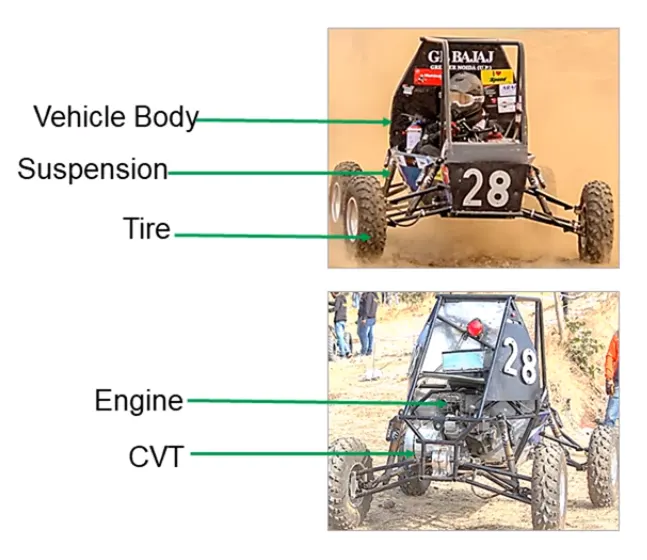
An ATV has the following main components

1. Vehicle body
2. Suspension
3. Tires
4. CVT
5. Engine

What is BAJA?

Basically Baja SAE is an intercollegiate design competition run by the Society of Automotive Engineers (SAE). Teams of students from universities all over the world design and build small off-road cars. The cars all have engines of the same specifications. As of 2018 the engine has been an unmodified Briggs & Stratton Model 19 Vanguard engine single-cylinder with a displacement of 305cc and power output of approximately 10 bhp (7.5 kW). In India, this event is run by SAE India.

There are multiple dynamic events, usually four per event, as well as a single four-hour endurance race. The dynamic events include hill climbs, sled pulls, manoeuvrability events, rock crawls, and suspension & traction events.

Static events, such as written reports, presentations and design evaluations are provided by participating teams. This is when the teams are judged on ergonomics, functionality, and producibility of their cars; ensuring that the final placement of the team does not rest solely on the vehicle's performance but rather on a combination of static and dynamic events. Required reports detail the engineering and design process that was used in developing each system of the team's vehicle, supported with sound engineering principles.

What is a CVT?

A continuously variable transmission (CVT), also known as a shiftless transmission, step-less transmission, pulley transmission, or, in case of motorcycles, a "twist-and-go", is an automatic transmission that can change seamlessly through a continuous range of effective gear ratios. This contrasts with other mechanical transmissions that offer a fixed number of gear ratios. The flexibility of a CVT with suitable control may allow the input shaft to maintain a constant angular velocity even as the output speed varies.

A belt-driven design offers approximately 88% efficiency, which, while lower than that of a manual transmission, can be offset by lower production cost and by enabling the engine to run at its most efficient speed for a range of output speeds. When power is more important than economy, the ratio of the CVT can be changed to allow the engine to turn at the RPM at which it produces greatest power. This is typically higher than the RPM that achieves peak efficiency. In low-mass low-torque applications (such as motor scooters) a belt-driven CVT also offers ease of use and mechanical simplicity.

A CVT does not strictly require the presence of a clutch. Nevertheless, in some vehicles (e.g. motorcycles), a centrifugal clutch is added to facilitate a "neutral" stance, which is useful when idling or manually reversing into a parking space.

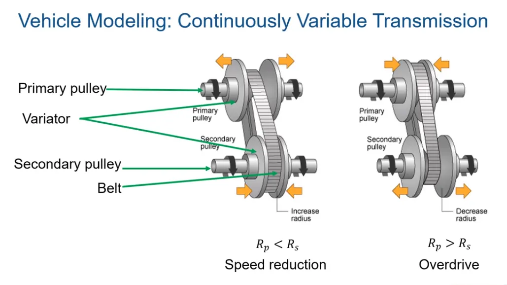
In CVT there are components namely Primary pulley, Secondary pulley, Variator and Belt. When the vehicle speed has to be reduced, the variator at primary side widen, reducing the primary radius while the variator at the secondary side gets compact which results in increasing the radius, thus the speed at secondary shaft reduces resulting in vehicle speed reduction.

When the vehicle speed has to be increased, the variator on the primary side gets compact resulting in increasing the primary radius while the variator at the secondary side widens which results in reduction of the secondary diameter which will finally result in increasing the secondary shaft which in turn increases the vehicle velocity.

Model description:

Now coming back to the Simulink and Simscape model which is the main point of discussion in this project. The model that is been described here is a simple model, whose sole purpose is to examine the behaviour of the vehicle and response to the throttle and brake input. This model cannot be compared to the real world ATV model as it does not take into account the suspension calculation and the calculation related to the tire model, since in this model we have considered the default wheel blocks. But, this model can definitely give an insight into the effect experienced by the ATV due to change in parameters such as mass value, gear ratio etc. Let us see a basic model for understanding.

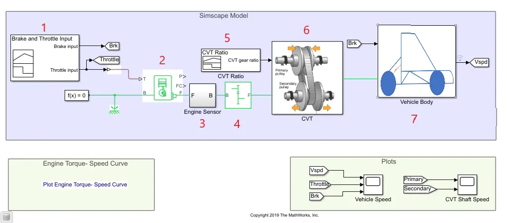
From the model, let us define some of the Simulink and Simscape blocks,

1. Signal builder - 1 – This block provides the input signals of the brake and throttle to respective subsystem or blocks. Here, throttle input is provide to ‘Generic Engine’ while the brake input is provided to ‘Vehicle body’ subsystem.
2. Generic Engine – This block represents a system-level model of spark-ignition and diesel engines suitable for use at initial stages of modeling when only the basic parameters are available.

The throttle input signal T lies between zero and one and specifies the torque demanded from the engine as a fraction of the maximum possible torque. If the engine speed falls below the Stall speed, the engine torque is blended to zero. If the engine speed exceeds the Maximum speed, the simulation stops and issues an error message.

Connections F and B are mechanical rotational conserving ports associated with the engine crankshaft and engine block, respectively. Connections P and FC are physical signal output ports through which engine power and fuel consumption rate are reported.

3. Engine Sensor – This is a subsystem containing rotational motion sensor which measures the rpm of the engine.
4. Simple Gear – This block connects the engine and the CVT which has a fixed gear ratio and this case the ratio is 4 between the base and follower.
5. Signal Builder-2 – This block provides the input signal to CVT subsystem for CVT ratio to be maintained during the simulation time of the model.
6. CVT Subsystem – This block provides the variation in the speed from input shaft to output shaft depending on the signal provided by the user in the signal builder-2.
7. Vehicle body subsystem – This system basically represents the total vehicle body to which engine power is provided through CVT. The break input is also provided to this subsystem.

Now, let’s understand what happens to this whole model when the simulation is ran in Simulink. Let’s observe the input provided in the form of throttle and break by the signal builder-1.

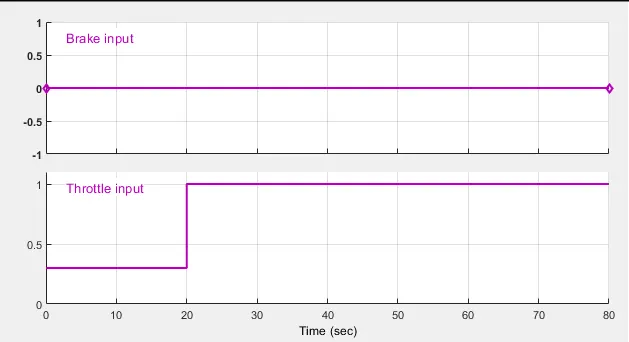
From the image it is understood that the simulation is ran for 80 sec and no brake is applied during this process and its value is 0 while the throttle is applied. Throttle value for the first 20 seconds is 0.3 and after that the throttle is increased upto 1. This signal is then provided to the ‘Generic engine’ block. But, the signal applied is in Simulink form and need to be converted into physical signal which is done using Simulink-PS converter

The ‘Generic Engine’ needs to be provided with the speed and torque value, if the engine speed and torque behaviour is known to us. Based on the throttle applied, necessary speed and torque output will be provided by the engine. In this model the relation between Speed and Torque can be observed as,

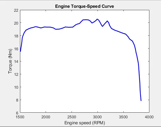
As can be observed from the graph, engine torque value is high and it increases until maximum speed is attained and then it starts to decrease and reaches to lower value at maximum engine speed. The maximum speed of the engine in this case 3840 rpm which is based on the engine specification and it’s built.

The input value of speed and torque are obtained from this curve and feed into the ‘Generic Engine’ block parameters in the form of the vector whose values can be seen in the MATLAB workspace.

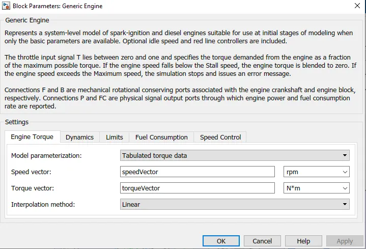
Based on the throttle applied corresponding torque and speed output is provided through ‘Engine Sensor’ subsystem to the ‘Simple Gear’ block where the speed value reduces due to gear ratio of 4. This reduced speed from the gear box is provided to the CVT block.

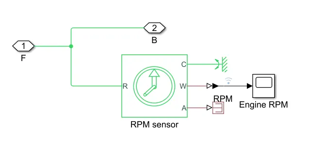
Engine Sensor subsystem

The speed at the primary shaft provided from the simple gear box is further varied depending on the CVT ratio applied by the Signal-Builder-2 and the corresponding speed can be observed at the output shaft. Rotational motion sensor are applied at each shaft to measure the input and output shaft speed. Let’s have a look at the CVT subsystem. From the CVT subsystem, the Inertia block represents the primary and secondary pulley. The input at primary is feed into Variable ratio gear drive which after variation can be obtained at the output shaft.

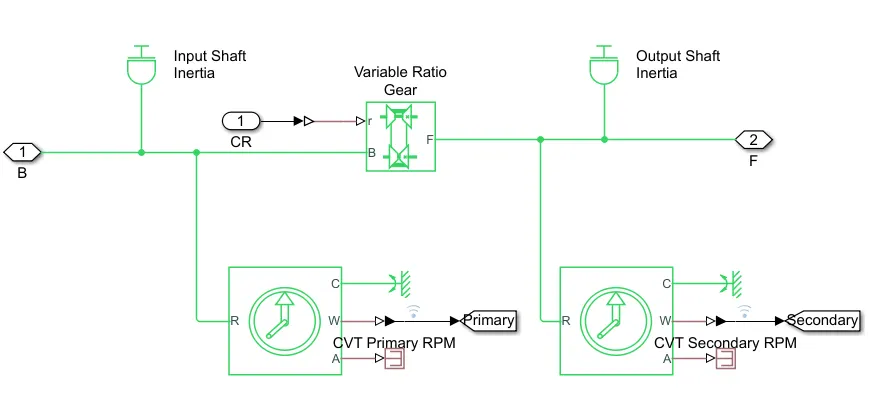
CVT subsystem

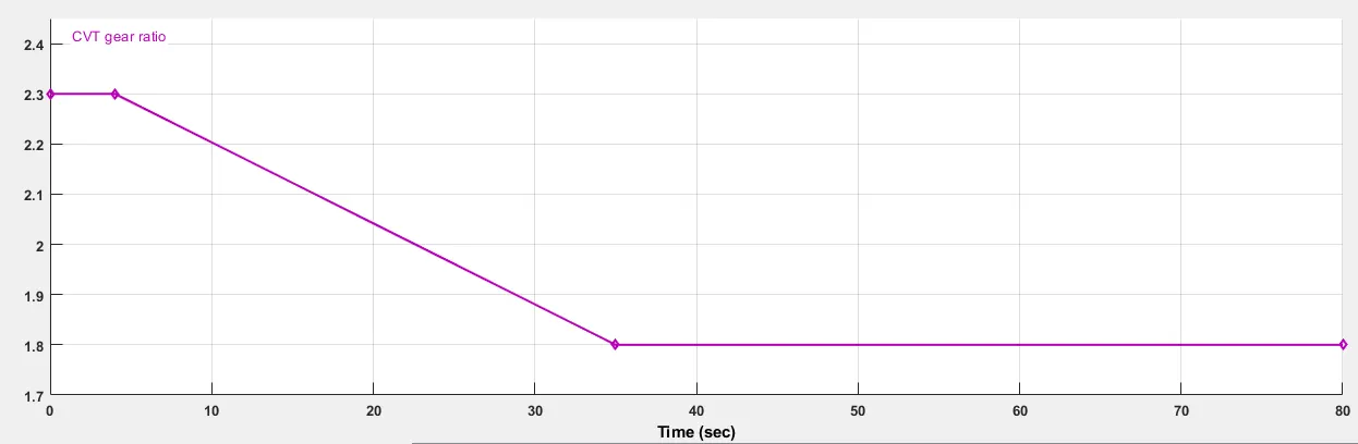
CVT ratio input from Signal Builder-2

The output speed of the CVT is then provided to the axel of the Vehicle body subsystem, which is then transferred to the wheels connected to the axels. The physical signal from the front and rear wheels are provided to the designated front and rear input port of the Vehicle Body block. Vehicle input block have been assigned certain variables such as mass of the body, number of wheels per axel, centre of gravity from front and rear axel and height from ground, also drag coefficient values can be entered into this block. This parameters play an important role in calculating the velocity of the ATV and its behaviour with the throttle input. When throttle is at its maximum, we will get the maximum velocity attained by the ATV. Brake input from Signal-Builder-1 is applied to the wheels of the vehicle body and depending on the signal obtained the vehicle will stop or remain in motion. In this model, no brakes are applied. Let’s observe the Vehicle Body subsystem.

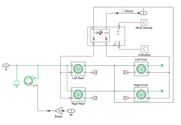
Vehicle Body Subsystem

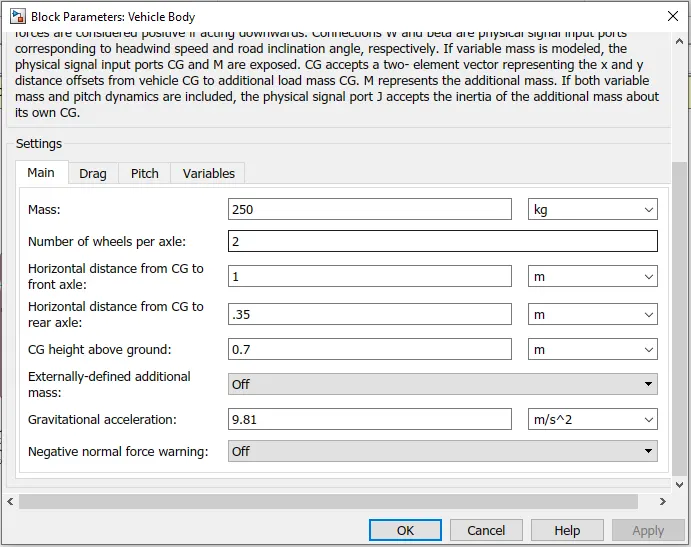
Vehicle Body Parameters

From the subsystem, we can understand that the output from the CVT is applied to the rear wheel blocks while the front wheels are free to rotate and an inertia block is also connected to imply the tires motion.

Brake input is first converted into physical signal with the help of Simulink-PS converter block which is then applied to the wheels through the Double-Shoe Brake block. The physical output signal from port ‘N’ of the wheel blocks are provided to the physical input port ‘NR’ and ‘NF’ of the Vehicle Body block. Any additional forces like air-drag and hill climb are also provided to the Vehicle Body, whose value are maintained 0 in this model.

The velocity of the system can be obtained from the physical output port ‘V’ of the Vehicle Body block. This signal is connected to the Scope through a PS-Simulink converter, the change in velocity with the change in applied throttle can be observed.

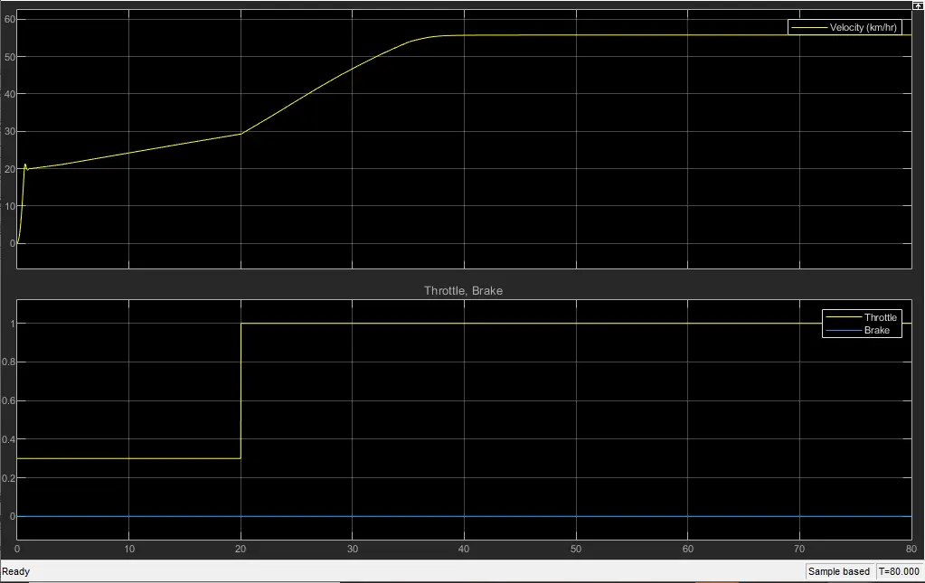
Plot of Change in velocity with change in Throttle input

From the plots it can be observed that, the velocity at the start steeply increases to a value of around 22 Kmph when an initial throttle of 0.3 is applied to the engine, the throttle remains nearly constant for 20 second during which the velocity steadily rises to 29 kmph. After 20 seconds, full throttle is given to the engine and the velocity again starts to rise up steeply to its maximum value of 55.7 kmph which is attained at 40 seconds count. From there the velocity remain constant till the simulation time ends. This is the maximum speed that can be attained by the vehicle.

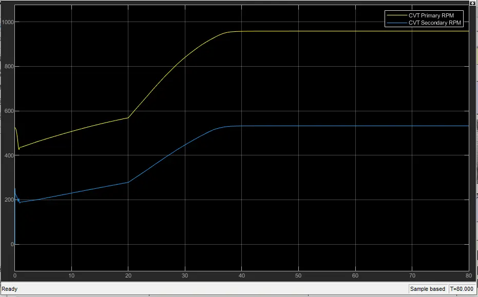
Primary and Secondary RPM

2] Now let us observe the second model with variable throttle and brake input,

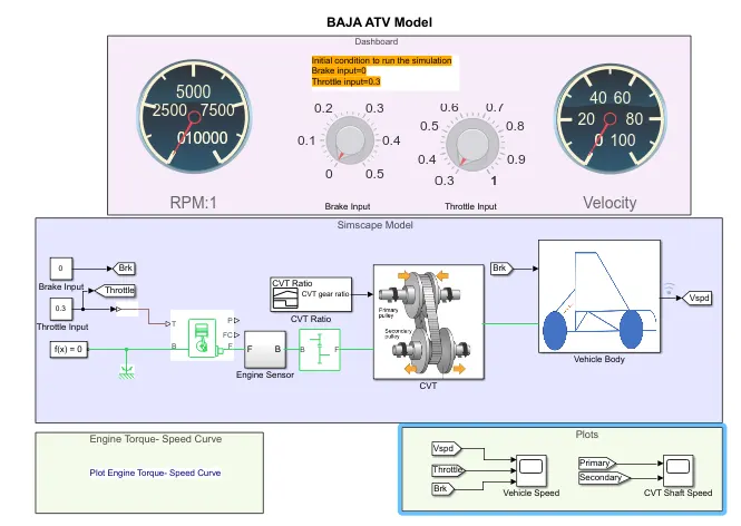
This model is same as the one discussed above, the only change in this model is the mode of inputs that are provided to the engine and vehicle i.e throttle and brake. The controls and the display in the model is similar to that of a car dashboard. In this model, the inputs are provided using a Knob block which can be rotated to increase or decrease the input values. Rest all the parameters are same and block connection are same.

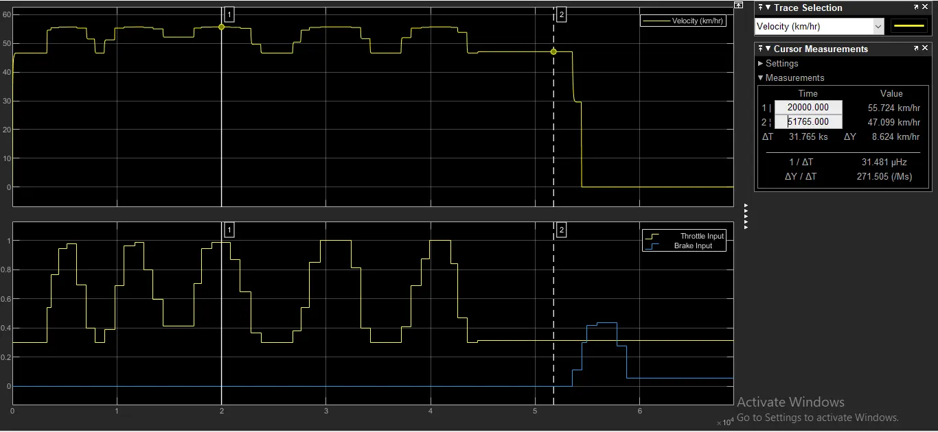
As in the case above, the initial value of throttle applied is 0.3 and brake value is 0. When the simulation is ran and at the initial value of the throttle, the velocity of the vehicle increases gradually and becomes constant at 47 kmph. If the throttle value is increased from 0.3 upto 1, the velocity of the vehicle also increases to a maximum value of 55.7 kmph, same as in the above model. As the throttle is increased and decreased simultaneously, the velocity also varies accordingly. In the end, throttle is brought to its original position and brake is applied causing the vehicle to stop and velocity becomes 0 kmph.

The plot of change in velocity with respect to change in throttle input is as follows,

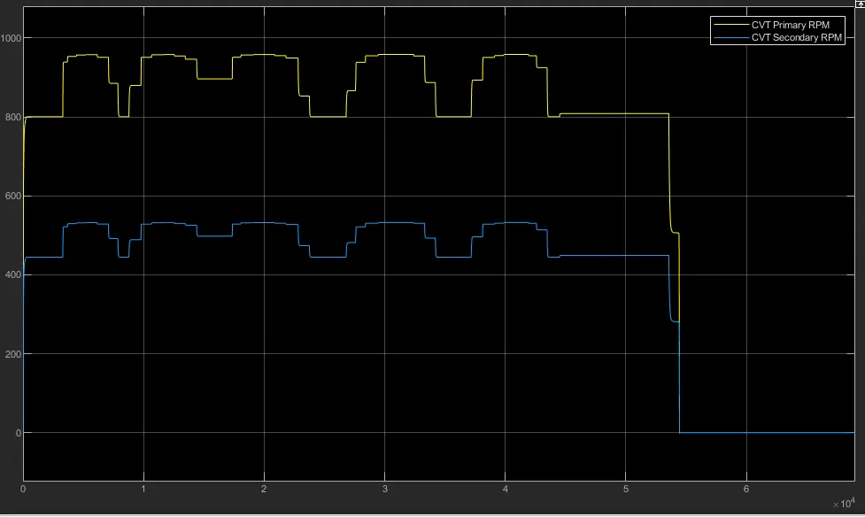
Plot for the Primary and Secondary RPM of the CVT,

The two models discussed above are said to be in open loop, as the input to the CVT are applied from an external source that have some random values. To avoid this and make the results more realistic, we have designed other model which is closed loop i.e the input to the CVT is based on the output velocity. This input is applied to the ‘Lookup Table’ block which will determine the CVT ratio corresponding to the applied velocity. The values in the Lookup Table are provided based on the results obtained in the open loop condition. The closed loop model provides more realistic results. Let’s have a look on the closed loop models.

3] Closed loop CVT driven ATV,

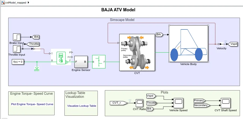
From the model it can be clearly that the Signal-Builder-1 block is replaced by two Step block each for the Brake and Throttle input. In this model also, the brake input does not have any significance as we are concerned with the main output i.e the velocity of the vehicle. Also, in this model Signal-Builder-2 block from the first model is removed and a signal from the output i.e velocity signal is feed back into the CVT block. Based on the feedback velocity value received, the CVT adjust its ratio referring the data of the Lookup Table and then varying the rpm accordingly. Rest of the block are maintained in same way as discussed in the above two models. Let’s observe the plot and understand the relation of the CVT ratio with the speed.

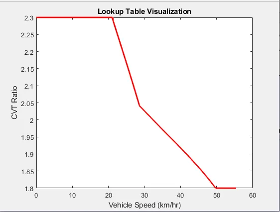
CVT ratio vs Speed

Now let’s have a look on the output velocity plot and the plot for the primary and secondary rpm of the CVT.

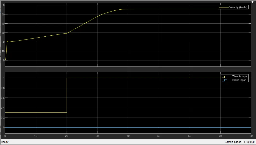
Change in Velocity due to change in throttle input

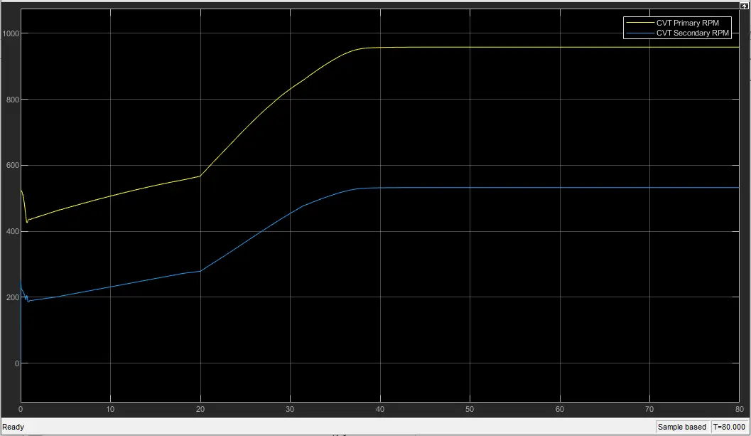
Primary and Secondary RPM changes according to throttle

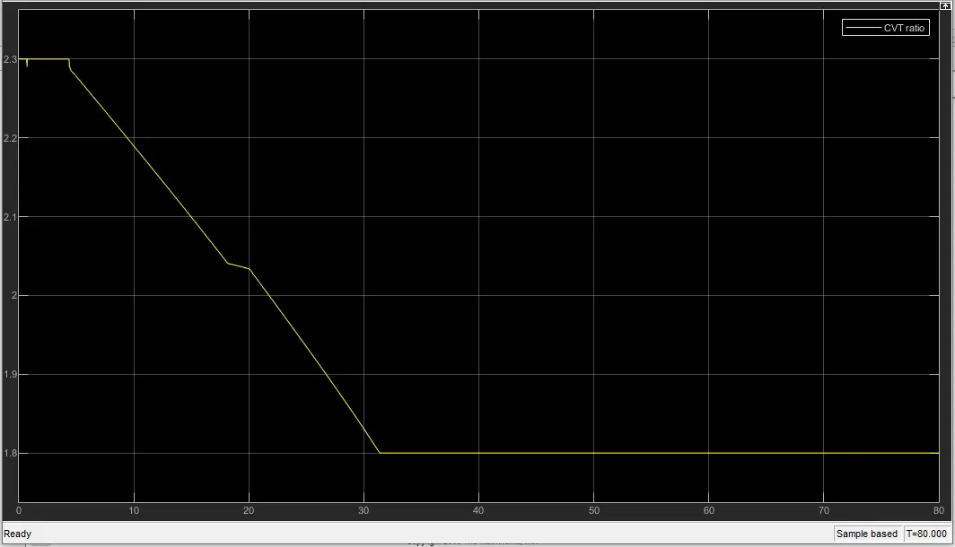
CVT ratio Changes according to Velocity feedback due to Throttle input

From the above plot it is clear that CVT ratio changes according to the feedback it receives from the output. At the start when the throttle is applied the velocity of vehicle increases and now this is feed back to the CVT, which in turn changes its ratio as the velocity keeps on increasing. As the velocity increases, the CVT ratio decreases. After 20 seconds, when the throttle value is switched to 1, the velocity increases and then the CVT ratio further decreases reaches to its lowest value and at that point the vehicle velocity reaches to its maximum value. Hence, this closed loop system is more realistic and useful than the open system. According to the changes in the CVT ratio, the primary and secondary speed also changes accordingly which can be seen in the above plot.

In the above model there was not much variation in the throttle input, the throttle was switched from 0.3 to 1. Now let us discuss the second model again, but this time the CVT ratio will change as per the close loop system. The velocity feedback is give the to the CVT block through the values defined in the Lookup Table for the specified velocity range.

4] Variable Throttle input provided to closed loop CVT driven ATV and the model can be seen as follows,

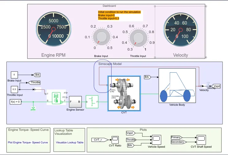
This model is similar to the second model discussed above, only change is the velocity feedback which will play huge role in adjusting the CVT ratio as per the demand. All the other components in the model remains the same. Now let us observe the output of the model,

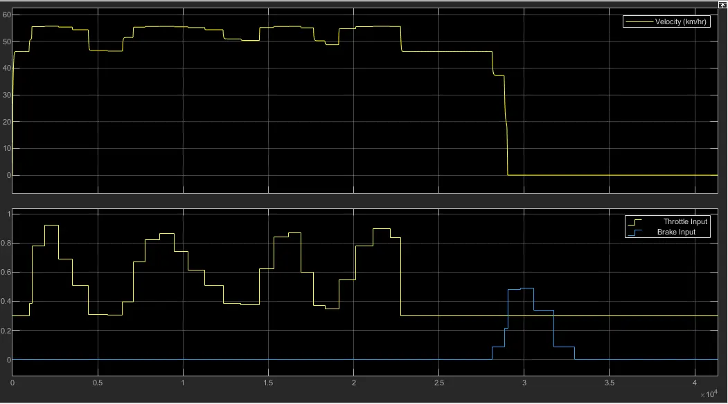
Change in velocity with the change in throttle input

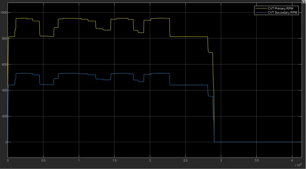
Primary and Secondary speed plot

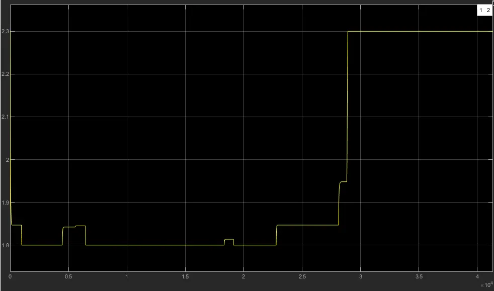
Variation in CVT ratio

From the above plot it can be seen that as the throttle value increases, the vehicle velocity also increases and vice versa. Initially the vehicle take some time to reach a nominal speed when the throttle of 0.3 is applied at the initial condition, from there the vehicle reaches to a specific speed and when the throttle is increased from that point the velocity also increases. When throttle is brought back to its initial condition so as to apply the brake, the vehicle stops as full brake gets applied.

The change in CVT ratio can be seen above and we can understand the variation in the ratio change, at start maximum CVT ratio is applied to bring the vehicle into motion until it attains a specific speed till that point the CVT ratio keeps on decreasing gradually. As the vehicle attain a specific speed and when the throttle is applied in order to increase the speed of vehicle to its optimum value, the CVT ratio decreases to its lowest value at which the vehicle speed will be maximum. When the throttle is decreased, the CVT ratio increases accordingly. Hence the output obtained is more realistic and practical.

Conclusion:

The BAJA ATV model was closely studied and all the results were understood for different arrangements made in the model.

All the behavioural characteristic of the vehicle related to the speed (velocity), CVT ratio, speed and torque relation and primary & secondary rpm were studied and understood.