Curve Fitting using Python

AIM: To create a program to perform curve fitting of a linear and cubic polynomial using Python

OBJECTIVE:

• To write a Python script to curve fitting of a linear and cubic polynomial
• To plot the actual data and the fitted curve to compare accuracy

INTRODUCTION

Curve Fitting:

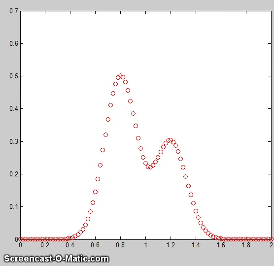
Curve fitting is the process of constructing a curve, or mathematical function, that has the best fit to a series of data points, possibly subject to constraints. Curve fitting can involve either interpolation, where an exact fit to the data is required, or smoothing, in which a "smooth" function is constructed that approximately fits the data.It involves finding a curve from a set of curves that best matches a series of data points. The set of curves is defined in terms of curve parameters. In other words, curve fitting consists of finding the curve parameters that produce the best match.

Types of curve fitting

Interpolation: where you discover a function that is an exact fit to the data points. Since this assumes no measurement error, it has limited applicability to real-life scenarios.

Smoothing: when we find a function that is an approximate fit to the data points, but we give room for error and we allow our actual points to be near, but not necessarily on the line; given the error is minimized overall.

Linear regression and Linear equations

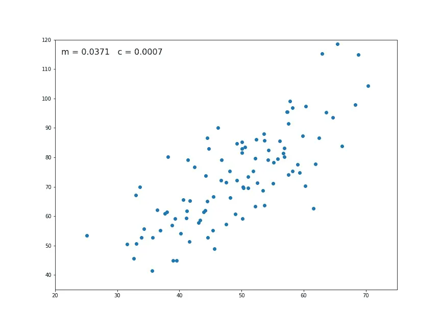
It is when the data is fit to a straight line. Although there might be some curve to your data, a straight line provides a reasonable enough fit to make predictions. Since the equation of a generic straight line is always given by `f(x)= ax+b`, the question becomes: what values of ‘a’ & ‘b’ will give us the best fit line for our data?Considering the vertical distance from each point to a prospective line as an error, and summing them up over our range, gives us a concrete number that expresses how far from ‘best’ the prospective line is. A line that provides a minimum error can be considered the best straight line.

Polynomial Regression and cubic polynomials

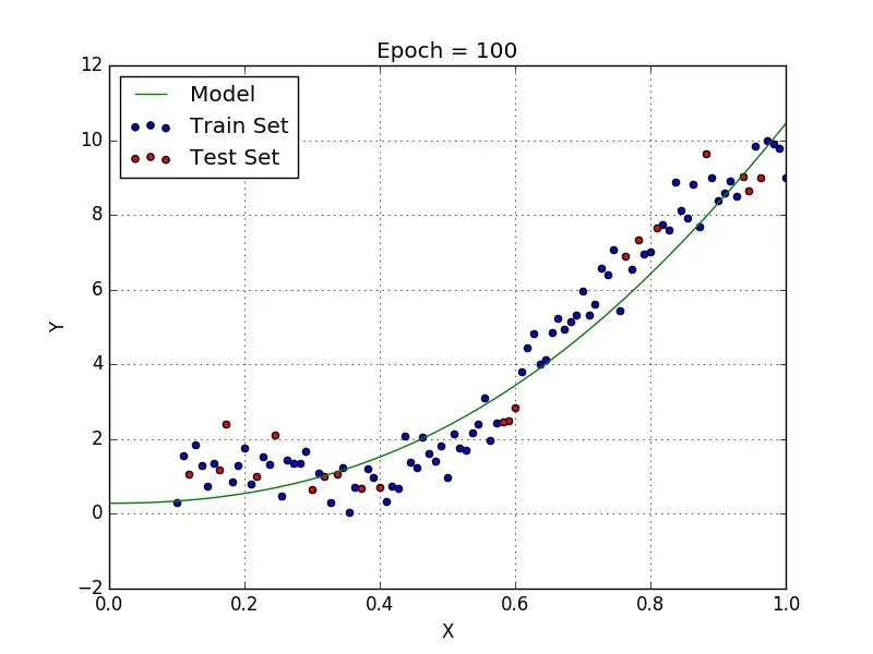
In statistics, polynomial regression is a form of regression analysis in which the relationship between the independent variable x and the dependent variable y is modelled as an nth degree polynomial in x. Polynomial regression fits a nonlinear relationship between the value of x and the corresponding conditional mean of y.Meanwhile, a cubic polynomial is a polynomial of degree 3. A univariate cubic polynomial has the form `f(x)=ax^3+bx^2+cx+d` . An equation involving a cubic polynomial is called a cubic equation. A closed-form solution known as the cubic formula exists for the solutions of an arbitrary cubic equation.

Equation used

• Linear equation: `xt+y`
• Cubic equation: `xt^3 + yt^2 + zt + d`

PROGRAM CODE

#Program to curve fit the cubic function  
#Importing the required modules and libraries
import numpy as np
import matplotlib.pyplot as plt 
from scipy.optimize import curve_fit

#Defining the necessary UDF's

#Linear Function
def lin_fun(t,x,y):
	return (x*t)+y
#Cubic Function
def cub_fun(t,x,y,z,xyz):
	return (x*pow(t,3)) + (y*pow(t,2)) + (z*t) + xyz  #Here cubic function is used as curve fit. 

#UDF for reading the thermodynamic data present in the file
def readfile(): 
	t = [] 
	cp = []
	for i in open('data', 'r'):
		x = i.split(',') 
		t.append(float(x[0])) 
		cp.append(float(x[1]))

	return [t, cp]

#MAIN PROGRAM
t, cp = readfile() 
popt, pcov = curve_fit(cub_fun, t, cp) #Curve fitting
fit_cp = cub_fun(np.array(t), *popt) #Here *popt contains the values for the constants present in our function or equation to be fitted.

#Plotting the curves 
plt.plot(t, cp,)
plt.plot(t, fit_cp,)
plt.legend(['Actual data','Curve fit'])
plt.xlabel('Temperature T (K)')
plt.ylabel('Specific heat C_p (J)')
plt.title("Curve fitting for a cubic function")
plt.savefig("CUBIC FUNCTION")
plt.show()

popt, pcov = curve_fit(lin_fun, t, cp) 
fit_cp = lin_fun(np.array(t), *popt) 


#Plotting the curves 
plt.plot(t, cp,)
plt.plot(t, fit_cp,)
plt.legend(['Actual data','Curve fit'])
plt.xlabel('Temperature T (K)')
plt.ylabel('Specific heat C_p (J)')
plt.title("Curve fitting for a linear function")
plt.savefig("LINEAR FUNCTION")
plt.show()


#Plot for comparison
popt1, pcov1 = curve_fit(lin_fun, t, cp) 
popt2, pcov2 = curve_fit(cub_fun, t, cp)
fit_cp_lin = lin_fun(np.array(t), *popt1)
fit_cp_cub = cub_fun(np.array(t), *popt2)
#Plotting the curves 
plt.plot(t, cp,)
plt.plot(t, fit_cp_lin,)
plt.plot(t, fit_cp_cub,)
plt.legend(['Actual data','Curve fit(Linear)','Curve fit(Cubic)'])
plt.xlabel('Temperature T (K)')
plt.ylabel('Specific heat C_p (J)')
plt.title("Comparing the curve fitting of linear and cubic fuctions with the orignal function")
plt.savefig("Comparison")
plt.show()

PROCEDURE

1. The neccesary libraries NumPy, Scipy.optimize.curve_fit, and matplotlib.pyplot are imported.
2. User-defined functions are created inorder to represent the linear and polynomial equation.
3. A user-defined function is also created for reading the neccesary thermodynamic data from the file 'data.txt'.
4. The respective curve fit functions are defined and the respective graphs are plotted.

RESULTS

OBSERVATIONS

From the graphs above, we can conclude that increasing the order of the polynomial, inturn improves the fitting of the curve withthe orignal data.

Questions

1. What does popt and pcov mean?

popt and pcov are parameters of Scipy.optimize.curve_fit Module.

popt: It is an array that provides an optimal value so that the sum of the squared residuals of the function. In general the return value ‘popt’ contains the best fit values of the parameters.

pcov: It contains the covariance matrix for the fit parameters. In general, the ‘pcov’ variable contains the covariance matrix, which indicates the uncertainties and correlations between parameters. This is most useful when the data has uncertainties.

2. What does np.array(temperature) do?

NumPy is used to work with arrays. The array object in NumPy is called ndarray. We can create a NumPy ‘ndarray’ object by using the array() function.

3. What does the * in *popt mean?

The star (*) is used as a reference or as an argument to a function. The star (*) notation will expand a list of values into the arguments of the function. This is useful if the function has more than one or two parameters. In general, the star (*) notation is used so that the variable which is placed after the star (*) is being referenced. The change occurred in the popt is reflected in the original popt value.

4. Write code to fit a linear and cubic polynomial for the Cp data. Explain if your results are good or bad.

The results for the cubic polynomila were good as we were able to fit that curve almost perfectly.The linear polynomial is obviously going to be a straight line and cannot be fitted perfectly

4. What needs to be done to make the curve fit perfectly?

The curve fit can never be perfect. The main reason for that is the actual Experimental value and the ideal curve-fit value always vary. However, the value of actual data may come close to the ideal curve fit value. This can be seen by the code and graph shown. As the order of the equations increase, the value gets closer to the ideal value.

RESULTS

Hence, using the above code, we were able to perform curve fitting on a Cubic polynomial.