Curve Fitting using MATLAB

AIM: To create a program to perform curve fitting of a linear and cubic polynomial using MATLAB

OBJECTIVE:

• To write a MATLAB program to curve fitting of a linear and cubic polynomial
• To plot the actual data and the fitted curve to compare accuracy
• To write a program to show the splitwise method.

INTRODUCTION

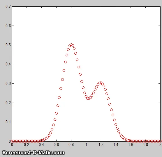
Curve Fitting:

Curve fitting is the process of constructing a curve, or mathematical function, that has the best fit to a series of data points, possibly subject to constraints. Curve fitting can involve either interpolation, where an exact fit to the data is required, or smoothing, in which a "smooth" function is constructed that approximately fits the data.It involves finding a curve from a set of curves that best matches a series of data points. The set of curves is defined in terms of curve parameters. In other words, curve fitting consists of finding the curve parameters that produce the best match.

Types of curve fitting

Interpolation: where you discover a function that is an exact fit to the data points. Since this assumes no measurement error, it has limited applicability to real-life scenarios.

Smoothing: when we find a function that is an approximate fit to the data points, but we give room for error and we allow our actual points to be near, but not necessarily on the line; given the error is minimized overall.

Linear regression and Linear equations

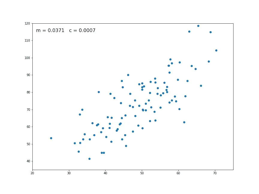
It is when the data is fit to a straight line. Although there might be some curve to your data, a straight line provides a reasonable enough fit to make predictions. Since the equation of a generic straight line is always given by `f(x)= ax+b`, the question becomes: what values of ‘a’ & ‘b’ will give us the best fit line for our data?Considering the vertical distance from each point to a prospective line as an error, and summing them up over our range, gives us a concrete number that expresses how far from ‘best’ the prospective line is. A line that provides a minimum error can be considered the best straight line.

Polynomial Regression and cubic polynomials

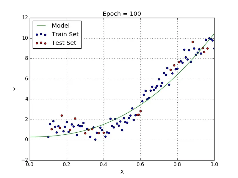
In statistics, polynomial regression is a form of regression analysis in which the relationship between the independent variable x and the dependent variable y is modelled as an nth degree polynomial in x. Polynomial regression fits a nonlinear relationship between the value of x and the corresponding conditional mean of y.Meanwhile, a cubic polynomial is a polynomial of degree 3. A univariate cubic polynomial has the form `f(x)=ax^3+bx^2+cx+d` . An equation involving a cubic polynomial is called a cubic equation. A closed-form solution known as the cubic formula exists for the solutions of an arbitrary cubic equation.

Equations

• Linear equation: `at+y`
• Cubic equation: `at^3 + bt^2 + ct + d`

PROGRAM CODE

Original Dataset

clc
close all
clear all
%Assigning the data in the file to a variable
cp_data=load('data');

%Splitting the data into their respective arrays
temp=cp_data(:,1);
cp=cp_data(:,2);


%Plotting
plot(temp,cp,'linewidth',3,'color','red')
xlabel('Temperature [K]')
grid on
title("Temperature VS Specific Heat")
ylabel('Specific Heat [KJ/Kmol-K]')

Program for linear and cubic curve fitting

clear all
close all
clc

%Assigning the data in the file to a variable
d=load('data');
%Splitting the data into their respective arrays
temp=d(:,1);  
cp=d(:,2);

%Linear Polynomial
[lin_coeff,s,mu]=polyfit(temp,cp,1);
cp_fit_lin=polyval(lin_coeff,temp,s,mu);

%Plotting
figure(1)
plot(temp,cp,'linewidth',2,'color','green');
hold on
plot(temp,cp_fit_lin,'linewidth',2,'color','red');
grid on
title("Linear Curve Fit")
xlabel('Temperature [K]')
ylabel('Specific Heat [KJ/Kmol-K]')
legend("Orignal","Linear Curve Fit")

%Cubic Polynomial
[cub_coeff,s,mu]=polyfit(temp,cp,3);
cp_fit_cub=polyval(cub_coeff,temp,s,mu);

%Plotting
figure(2)
plot(temp,cp,'linewidth',2,'color','green');
hold on
plot(temp,cp_fit_cub,'linewidth',2,'color','blue');
grid on
title("Cubic Curve Fit")
xlabel('Temperature [K]')
ylabel('Specific Heat [KJ/Kmol-K]')
legend("Orignal","Cubic Curve Fit")

Improving the cubic fit using Splitwise Curve Fit

Splitwise Curve Fit

clear all
close all
clc

%Assigning the data in the file to a variable
d=load('data');
%Splitting the data into their respective arrays
temp=d(:,1);  
cp=d(:,2);

%Dividing the data into 4 parts

%Part 1
temp1=d(1:460,1);
cp1=d(1:460,2);

%Part 2
temp2=d(461:1100,1);
cp2=d(461:1100,2);

%Part 3
temp3=d(1101:2200,1);
cp3=d(1101:2200,2);

%Part 4
temp4=d(2201:3200,1);
cp4=d(2201:3200,2);


%Cubic Curve 

%Part 1
[cp_coeff1,s1,mu1]=polyfit(temp1,cp1,3);
cp1_fit_cub1=polyval(cp_coeff1,temp1,s1,mu1);

%Part 2
[cp_coeff2,s2,mu2]=polyfit(temp2,cp2,3);
cp1_fit_cub2=polyval(cp_coeff2,temp2,s2,mu2);

%Part 3
[cp_coeff3,s3,mu3]=polyfit(temp3,cp3,3);
cp1_fit_cub3=polyval(cp_coeff3,temp3,s3,mu3);

%Part 4
[cp_coeff4,s4,mu4]=polyfit(temp4,cp4,3);
cp1_fit_cub4=polyval(cp_coeff4,temp4,s4,mu4);

%Plotting
plot(temp,cp,'linewidth',5,'color','black')
hold on 
plot(temp1,cp1_fit_cub1,'color','r','linewidth',2)
plot(temp2,cp1_fit_cub2,'color','b','linewidth',2)
plot(temp3,cp1_fit_cub3,'color','g','linewidth',2)
plot(temp4,cp1_fit_cub4,'color','y','linewidth',2)
hold off
grid on
title("Cubic Splitwise Curve Fit")
xlabel('Temperature [K]')
ylabel('Specific Heat [KJ/Kmol-K]')
legend("Orignal","Cubic Curve Fit Part 1","Cubic Curve Fit Part 2","Cubic Curve Fit Part 3","Cubic Curve Fit Part 4")

The curves completely overlap.Orignal curve's thickness is increased to differentiate between the orignal curve and splitwise curve

How to get the perfect fit:

In order to make perfect fit, we must consider error estimates as well. Perfect fit means, the curve should fit the original curve without showing any errors (such as centering and scaling erros) in that perticular degree of polynomial. Perfect fit can always be a best fit but best fit can not be a perfect fit. So, in the 3rd order polynomial I have eliminated the errors, that means curve fit we got using 'Linear regression witherror estimates' is perfect fit for 3rd order polynomial. But it is still not the best fit. To calculate best fit, we must increase the order or use splitwise method.

How to get the best fit:

For this, we can use RMS(Root Mean square) or simple linear regression. We can change the order of polynomial to get the perfect fit. ANd the best way is, split the data in two or more data folds and do the curve fit. I have shown how to make a best fit using 3rd order polynomial in the last part of the project. If we use, changing od polynomial order method to get the curve fit, then 9th order is the best fit. But, in split-wise method that I have shwon at the bottom, even the 3rd order can give the best fit.

How to make a curve fit perfectly?

Using an iterative method by increasing the order of the equation.

ERRORS ENCOUNTERED AND ELIMINATING THEM

Inorder to eliminate this error, we have to use centering and scaling.

When we use the 'polyfit' command, while calculating the coefficients, we need to calculate error estimation structure (s) and centering and scaling values (mu), to avoid the error above.

CONCLUSION

Hence, using the above program we were able to perform a curve fitting for a linear and cubic polynomial for the Cp data and also measure the fitness characteristics for both the curves.