CURVE FITTING OF DATA
CURVE FITTING
AIM: To find the coefficients of linear, quadratic and cubic polynomial and draw the corresponding fit
PROGRAM:
CASE1: COMPARISON OF SPLITWISE FIT WITH CUBIC FIT METHOD
clear all

close all

clc


%PREPARING THE DATA

cp_data=load('data')%LOAD DATA FROM THE SYSTEM

temperature=cp_data(:,1)% EXTRACT THE VALUE OF TEMPERATURE FROM THE LOADED DATA'cp_data'

cp=cp_data(:,2)% EXTRACT THE VALUE OF SPECIFIC HEAT CAPACITY FROM THE LOADED DATA'cp_data'


%CURVE FIT

%LINEAR EQUATION==>cp=a*T+b

% co_ef=polyfit(temperature,cp,1);%FINDING THE COEFICIENTS FOR LINEAR EQUATION

% predicted_cp3=polyval(co_ef,temperature);%CALCULATE THE VALUE OF CORRESPONDING SPECIFIC HEAT


%cp=a*T^2+b*T+C


co_ef=polyfit(temperature,cp,2);%FINDING THE COEFICIENTS FOR QUDRATIC EQUATION

predicted_cp=polyval(co_ef,temperature);%CALCULATE THE VALUE OF CORRESPONDING SPECIFIC HEAT


%cp=a*T^3+b*T^2+C*T+D


co_ef=polyfit(temperature,cp,3);%FINDING THE COEFICIENTS FOR CUBIC EQUATION

predicted_cp2=polyval(co_ef,temperature);%CALCULATE THE VALUE OF CORRESPONDING SPECIFIC HEAT


%%SPLITWISE CURVE FITTING METHOD

%%THIS INCLUDE SPLITTING THE DATABASE ACCORDING TO THE VARIATION OF DATA IN

%%THE CHANGE IN THE CHARACTERISTICS OF THE DATA


temp01= temperature(1:400);

cp01=cp(1:400);

coeff01=polyfit(temp01,cp01,1);

predicted_cp01=polyval(coeff01,temp01);


temp02=temperature(401:800);

cp02=cp(401:800);

coeff02=polyfit(temp02,cp02,2);

predicted_cp02=polyval(coeff02,temp02);


temp03=temperature(801:1200);

cp03=cp(801:1200);

coeff03=polyfit(temp03,cp03,2);

predicted_cp03=polyval(coeff03,temp03);


temp04=temperature(1201:1600);

cp04=cp(1201:1600);

coeff04=polyfit(temp04,cp04,2);

predicted_cp04=polyval(coeff04,temp04);


temp05=temperature(1601:2000);

cp05=cp(1601:2000);

coeff05=polyfit(temp05,cp05,2);

predicted_cp05=polyval(coeff05,temp05);


temp06=temperature(2001:2400);

cp06=cp(2001:2400);

coeff06=polyfit(temp06,cp06,2);

predicted_cp06=polyval(coeff06,temp06);


temp07=temperature(2401:2800);

cp07=cp(2401:2800);

coeff07=polyfit(temp07,cp07,1);

predicted_cp07=polyval(coeff07,temp07);


temp08=temperature(2801:3200);

cp08=cp(2801:3200);

coeff08=polyfit(temp08,cp08,1);

predicted_cp08=polyval(coeff08,temp08);


predicted_cp_comb=[predicted_cp01;predicted_cp02;predicted_cp03;predicted_cp04;predicted_cp05;predicted_cp06;predicted_cp07;predicted_cp08]


%CALCULATING FITNESS CHARACTERS

pred_cp_mean=mean(predicted_cp_comb);

SSR=sum((predicted_cp_comb-pred_cp_mean).^2);

error=predicted_cp_comb-cp;

SSE=sum(error.^2);

SST=(SSR+SSE);%SUM OF SQUARE OF TOTAL

r_sq=(SSR/SST);

r_perc=r_sq*100;

split_char=table(SSE,SSR,SST,r_sq,'VariableNames',{'SSE','SSR','SST','r SQUARED'})


%CALCULATING FITNESS CHARACTERS

pred_cp2_mean=mean(predicted_cp2);

SSR2=sum((predicted_cp2-pred_cp2_mean).^2);

error2=predicted_cp2-cp;

SSE2=sum(error2.^2);

SST2=(SSR2+SSE2);%SUM OF SQUARE OF TOTAL


r_sq2=(SSR2/SST2);

r_perc2=r_sq2*100;

cubic_char=table(SSE2,SSR2,SST2,r_sq2,'VariableNames',{'SSE','SSR','SST','r SQUARED'})


if r_sq>0.95

    fprintf('Split wise Cubic curve predicts %0.f percentage of correction from actual value',r_perc)

else

    disp('Split wise Cubic curve doesnot produce a best fit. Change the order or the split data series further')

end


%compare my curve fit with original data

plot(temperature,cp,'linewidth',3,'color','g') %PLOT THE ORIGINAL DATA

hold on

plot(temperature,predicted_cp_comb,'linewidth',3,'color','r')

% plot(temperature,predicted_cp,'linewidth',3,'color','r')%PLOT THE QUADRATIC FORM OF EQN

 hold on

 plot(temperature,predicted_cp2,'linewidth',3,'color','b')%PLOT THE CUBIC FORM OF EQN

% hold on

% plot(temperature,predicted_cp3,'linewidth',3,'color','k')%PLOT THE LINEAR FOR OF EQN

%

xlabel('Temperature')%LABEL X COMPONENT

ylabel('Specific Heat(KJ/kmol K')%LABEL Y COMPONENT

legend('Original dataset','Splitwise curve fitting','Third order fit')%LEGEND THE GIVEN DATA
CASE 2: COMPARISON OF LINEAR SPLITWISE FIT WITH CUBIC FIT
clear all

close all

clc


%PREPARING THE DATA

cp_data=load('data')%LOAD DATA FROM THE SYSTEM

temperature=cp_data(:,1)% EXTRACT THE VALUE OF TEMPERATURE FROM THE LOADED DATA'cp_data'

cp=cp_data(:,2)% EXTRACT THE VALUE OF SPECIFIC HEAT CAPACITY FROM THE LOADED DATA'cp_data'


%CURVE FIT

%LINEAR EQUATION==>cp=a*T+b

% co_ef=polyfit(temperature,cp,1);%FINDING THE COEFICIENTS FOR LINEAR EQUATION

% predicted_cp3=polyval(co_ef,temperature);%CALCULATE THE VALUE OF CORRESPONDING SPECIFIC HEAT


%cp=a*T^2+b*T+C


co_ef=polyfit(temperature,cp,2);%FINDING THE COEFICIENTS FOR QUDRATIC EQUATION

predicted_cp=polyval(co_ef,temperature);%CALCULATE THE VALUE OF CORRESPONDING SPECIFIC HEAT


%cp=a*T^3+b*T^2+C*T+D


co_ef=polyfit(temperature,cp,3);%FINDING THE COEFICIENTS FOR CUBIC EQUATION

predicted_cp2=polyval(co_ef,temperature);%CALCULATE THE VALUE OF CORRESPONDING SPECIFIC HEAT


%%SPLITWISE CURVE FITTING METHOD

%%THIS INCLUDE SPLITTING THE DATABASE ACCORDING TO THE VARIATION OF DATA IN

%%THE CHANGE IN THE CHARACTERISTICS OF THE DATA


temp01= temperature(1:400);

cp01=cp(1:400);

coeff01=polyfit(temp01,cp01,1);

predicted_cp01=polyval(coeff01,temp01);


temp02=temperature(401:800);

cp02=cp(401:800);

coeff02=polyfit(temp02,cp02,1);

predicted_cp02=polyval(coeff02,temp02);


temp03=temperature(801:1200);

cp03=cp(801:1200);

coeff03=polyfit(temp03,cp03,1);

predicted_cp03=polyval(coeff03,temp03);


temp04=temperature(1201:1600);

cp04=cp(1201:1600);

coeff04=polyfit(temp04,cp04,1);

predicted_cp04=polyval(coeff04,temp04);


temp05=temperature(1601:2000);

cp05=cp(1601:2000);

coeff05=polyfit(temp05,cp05,1);

predicted_cp05=polyval(coeff05,temp05);


temp06=temperature(2001:2400);

cp06=cp(2001:2400);

coeff06=polyfit(temp06,cp06,1);

predicted_cp06=polyval(coeff06,temp06);


temp07=temperature(2401:2800);

cp07=cp(2401:2800);

coeff07=polyfit(temp07,cp07,1);

predicted_cp07=polyval(coeff07,temp07);


temp08=temperature(2801:3200);

cp08=cp(2801:3200);

coeff08=polyfit(temp08,cp08,1);

predicted_cp08=polyval(coeff08,temp08);


predicted_cp_comb=[predicted_cp01;predicted_cp02;predicted_cp03;predicted_cp04;predicted_cp05;predicted_cp06;predicted_cp07;predicted_cp08]


%CALCULATING FITNESS CHARACTERS

pred_cp_mean=mean(predicted_cp_comb);

SSR=sum((predicted_cp_comb-pred_cp_mean).^2);

error=predicted_cp_comb-cp;

SSE=sum(error.^2);

SST=(SSR+SSE);%SUM OF SQUARE OF TOTAL

r_sq=(SSR/SST);

r_perc=r_sq*100;

split_char=table(SSE,SSR,SST,r_sq,'VariableNames',{'SSE','SSR','SST','r SQUARED'})


%CALCULATING FITNESS CHARACTERS

pred_cp2_mean=mean(predicted_cp2);

SSR2=sum((predicted_cp2-pred_cp2_mean).^2);

error2=predicted_cp2-cp;

SSE2=sum(error2.^2);

SST2=(SSR2+SSE2);%SUM OF SQUARE OF TOTAL


r_sq2=(SSR2/SST2);

r_perc2=r_sq2*100;

cubic_char=table(SSE2,SSR2,SST2,r_sq2,'VariableNames',{'SSE','SSR','SST','r SQUARED'})


if r_sq>0.95

    fprintf('Split wise Cubic curve predicts %0.f percentage of correction from actual value',r_perc)

else

    disp('Split wise Cubic curve doesnot produce a best fit. Change the order or the split data series further')

end


%compare my curve fit with original data

plot(temperature,cp,'linewidth',3,'color','g') %PLOT THE ORIGINAL DATA

hold on

plot(temperature,predicted_cp_comb,'linewidth',3,'color','r')

% plot(temperature,predicted_cp,'linewidth',3,'color','r')%PLOT THE QUADRATIC FORM OF EQN

 hold on

 plot(temperature,predicted_cp2,'linewidth',3,'color','b')%PLOT THE CUBIC FORM OF EQN

% hold on

% plot(temperature,predicted_cp3,'linewidth',3,'color','k')%PLOT THE LINEAR FOR OF EQN

%

xlabel('Temperature')%LABEL X COMPONENT

ylabel('Specific Heat(KJ/kmol K')%LABEL Y COMPONENT

legend('Original dataset','Splitwise curve fitting','Third order fit')%LEGEND THE GIVEN DATA
PRINCIPLE :
In the current problem, it deals with finding the fit for
Curve Fit: The process of constructing curve or a mathematical function from a series of data points. It also deals with Derive the relation between the independent variable(eg.x) to the dependent variable(e.g. y).
In the present study we plot the linear and cubic fit and compare the results of both.
Linear curve
First degree polynomial equation is y=ax+b
Where a is the slope of the line. It is an exact fit through any two points with distinct x coordinates. Here the order of polynomial is 1 and the no of unknown=2(a,b).i.e. number of unknows is always 1 greater than the order of the polynomial.
Cubic Curve
Third order polynomial equation used is y= ax3+bx2+cx+d. Here the order of polynomial is 3 and the number of unknows (a,b,c,d). Hence curve fitting a third order equation gives more accurate results compared to linear curve.
Since it is required to cubic fit the given set of values we initialize the variable cp_coeff and gives the order of polynomial as 3. cp_coeff contains variables of 4 unknows.
RESULTS
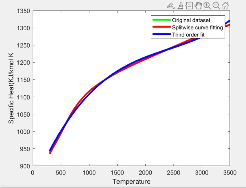
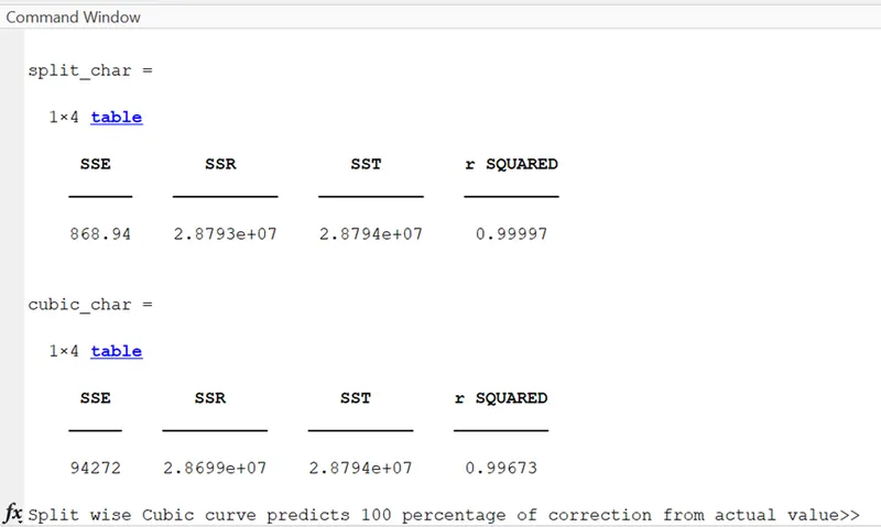
In the given task it is asked to find the curve fit of a given data using split wise fit and cubic fit.
CASE1
CASE2
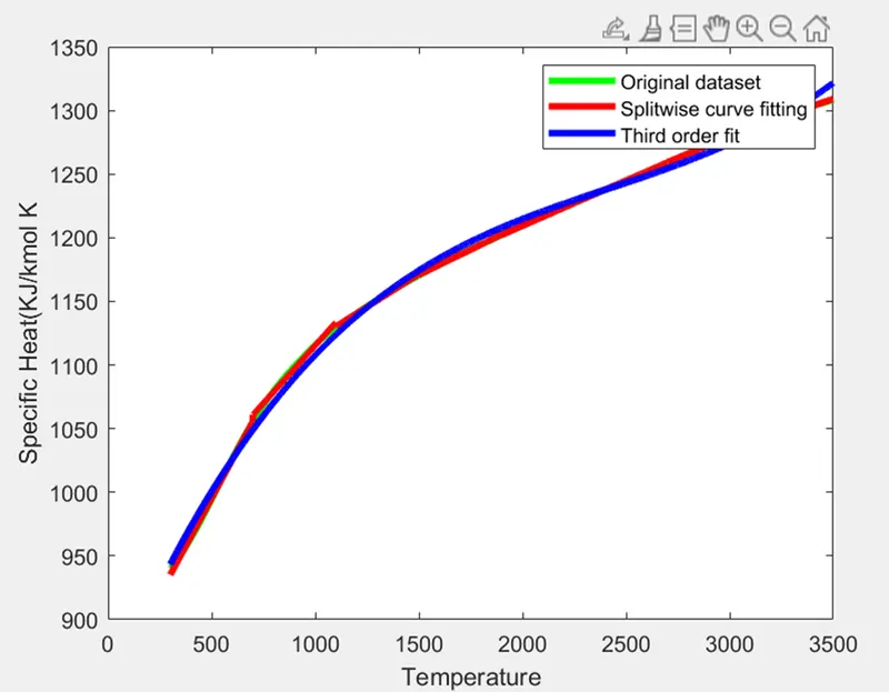
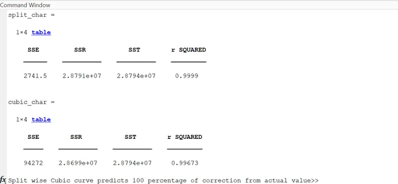
As observed the cubic fit posses less accuracy when compared with multiple splitwise fit. Hwncw we can say that the best method for finding the fitness of a given data is splitwise data
PERFECT FIT VS BEST FIT
Consider a system of n data points. Each data point might be a value of x and y where y is a function x. On curve fitting the given set of values, the curve obtained may be deviated from the actual values. These deviation from the actual value is called the error.