Curve Fit for linear and cubic polynomial equation.

CURVE FIT

Curve fitting is a process of contructing a curve or mathematical function that best fits to series of data points,subjected to constraints.It can either involve interpolation or extrapolation.

Interpolation: here an exact fit to the data is required,in other words,a smooth function is constructed that approximately fits the data.

Extrapolation:It uses an already fitted curve beyond the data range and a certain level of uncertainity is observed.

The first step in constructing a mathematical model is to plot these data ponts and postulate a function form f(x) to describe the general trend in data.

Some simple functions commonly used to fit data are:

• straight line: f(x) = ax + b
• parabola: f(x) = ax2 + bx + c
• polynomial: f(x) = = amx^m + am−1x^(m−1 )+ · · · + a2x^2 + a1x + a0

The coefficients a, b, c etc. in the formula of f(x) are parameters that we can adjust.

So,once we have a curve fit based on a polynomial equation,how do we determine it closeness to the original fit?

Well,There are many factors that affect the goodness of fit. By shere increase of the degree of polynomial we can improvise the fit to great extent,but other factors involved are:

1.Sum of squares due to error(SSE).

2.Root Mean Squared Error(RMSE).

3. R-square

4.Adjusted R-square.

SSE:

SSE is sum of squared deviation of actual from predicted values.

if SSE=0, predicted fit=original fit.

If SSE is high, not a good fit.

R-square:

Rsquare =SSR/SST, where SST=SSE+SSR .

SSR is sum of squared regression.

R>0.7 is considered for best fit

RMSE:

It is the square root of variance of residuals.It indicates the absolute fit of the model to the data.Lower values of RMSE indicate a good fit.

Here is a program to find the linear and cubic curve fit.

%Curve fit
close all
clear all
clc

cp_data=load('data','-ascii');
temperature=cp_data(:,1);
cp=cp_data(:,2);

%Linear curve fit
co_eff_L= polyfit(temperature,cp,1);
predicted_cp_L= polyval(co_eff_L,temperature);

%Cubic polynomial curve fit
co_eff_c=polyfit(temperature,cp,3);
predicted_cp_c=polyval(co_eff_c,temperature);

n=3200;
%Error calculation for predicted linear and cubic polynomial
error_L= cp-predicted_cp_L;
SSE_L= sum(error_L.^2);
SSR_L= sum((predicted_cp_L-mean(cp)).^2);
SST_L=SSR_L+SSE_L;
RSquare_L = SSR_L/SST_L;
RMSE_L=sqrt(SSE_L/n);

error_c= cp-predicted_cp_c;
SSE_c= sum(error_c.^2);
SSR_c= sum((predicted_cp_c-mean(cp)).^2);
SST_c=SSR_c+SSE_c;
RSquare_c = SSR_c/SST_c;
RMSE_c=sqrt(SSE_c/n);

%plotting
figure(1)
plot(temperature,cp,'linewidth',3','color','r');
hold on
plot(temperature,predicted_cp_L,'linewidth',3,'color','g');
plot(temperature,predicted_cp_c,'linewidth',3,'color','b');
title('Temperature Vs Specific heat');
xlabel('temperature[K]')
ylabel('SpecificHeat[KJ/Kmol-k]')
legend('Original dataset','Linear','Cubic');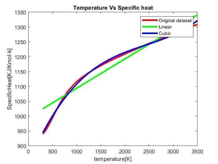

Explanation:

The file"data" is loaded using the load command which contains values oftemperature and specific heat.

Plotting the values of temp vs cop gives us the original dataset.

Using polyfit and polyval commands, the coefficients of the polynomial equation and predicted cp is determined.

plotting this would result in a curve fit. we can improve the fit by increasing the degree if polynomial.

To understand the goodness of fit, we dtermine the error using the formula availableand determine the fit. the higher degree equation(cubic) gives a better fit.

Splitwise Method

close all 
clear all
clc

%Inputs
cp_data=load('data','-ascii');
temp=cp_data(:,1);
cp=cp_data(:,2);
a=1;
n=3200;
b=320;
s=10;

% Splitwise method for Cubic polynomial
for i=1:s
   temp_i=cp_data((a:b),1);
   cp_i=cp_data((a:b),2);
   hold on
   plot(temp_i,cp_i,'linewidth',3,'color','r');
   plot(temp,cp,'linewidth',2,'color','b');
 
    coeff_i=polyfit(temp_i,cp_i,3);
    pred_i=polyval(coeff_i,temp_i);
    a=b;
    b=b+n/s;
   
end
 title('Temperature Vs Specific heat');
xlabel('temperature[K]')
ylabel('SpecificHeat[KJ/Kmol-k]')
legend('Predicted Cubic curve','Original dataset');

Explanation:

Load the data using load command. it contains data of temperature and specific heat.

obtain individual data of temp and cp.

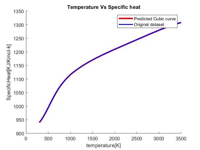
To get a closer fit,we are using splitwise method.Here we are dividing the datapoints(n=3200) into 10 divisions(s=10).

initialise the range operators a and b to 1 and 320 respectively.

using a for for loop with 10 iterations we have obtained 10 values of coeff,pred values. this is plotted in a graph to obtain the cubic curve fit.

Errors faced while coding:

Assigning the range operator was little difficult.

after assigning variables a and b, and incrementing it by 320, this issue was resolved.

i was thinking of adding all the individual divisions(10)to a matrix and later plot them,however i was not able to find a function that could store matrices into a array and later plot them.(please let me know if there are functions to store matrices and plot them if there are any in comment section).

however, plotting individual divisions along with hold on command solved the problem.

1.How to make a curve fit perfectly?

By increasing the order of the polynomial, we can obtain perfect fit. Also using stepwise method results in a fit close to original fit.

2.How to get best fit?

There are 4 quantities that determine the goodness of fit.they are:

Sum of Squares due to error,Rsquare,Adjusted R Square,Root mean squared error.

If Rsquare is close to 1(>0.95) it is considered as best fit.

3.Improve cubic fit?

cubic fit closely represents the original data. however using stepwise method results in a much better fit.

References:

http://www.dam.brown.edu/people/alcyew/handouts/leastsq.pdf

https://web.maths.unsw.edu.au/~adelle/Garvan/Assays/GoodnessOfFit.html